import pandas as pd
import matplotlib.pyplot as plt
from pandas.core.common import random_state
from sklearn.datasets import load_wine
= load_wine()
wine_load = pd.DataFrame(wine_load.data, columns=wine_load.feature_names)
wine 'class'] = wine_load.target
wine['class'] = wine['class'].map({0: 'class_0', 1: 'class_1', 2: 'class_2'})
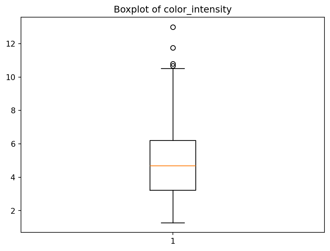
wine[
'color_intensity'], whis=1.5)
plt.boxplot(wine['Boxplot of color_intensity')
plt.title( plt.show()
데이터 전처리
데이터 분석
데이터 전처리의 의미
- 데이터 클리닝
- 데이터 통합
- 데이터 변환
- 데이터 축소
- 불균형 데이터 처리
- 데이터 분할
이상치 확인 및 정제
이상치 확인
import numpy as np
def outliers_iqr(dt, col):
= np.percentile(dt[col], [25, 75])
q1, q3 = q3 - q1
iqr = q1 - (iqr * 1.5)
lower_bound = q3 + (iqr * 1.5)
upper_bound return dt[(dt[col] < lower_bound) | (dt[col] > upper_bound)]
= outliers_iqr(wine, 'color_intensity')
outliers outliers
alcohol | malic_acid | ash | alcalinity_of_ash | magnesium | total_phenols | flavanoids | nonflavanoid_phenols | proanthocyanins | color_intensity | hue | od280/od315_of_diluted_wines | proline | class | |
---|---|---|---|---|---|---|---|---|---|---|---|---|---|---|
151 | 12.79 | 2.67 | 2.48 | 22.0 | 112.0 | 1.48 | 1.36 | 0.24 | 1.26 | 10.80 | 0.48 | 1.47 | 480.0 | class_2 |
158 | 14.34 | 1.68 | 2.70 | 25.0 | 98.0 | 2.80 | 1.31 | 0.53 | 2.70 | 13.00 | 0.57 | 1.96 | 660.0 | class_2 |
159 | 13.48 | 1.67 | 2.64 | 22.5 | 89.0 | 2.60 | 1.10 | 0.52 | 2.29 | 11.75 | 0.57 | 1.78 | 620.0 | class_2 |
166 | 13.45 | 3.70 | 2.60 | 23.0 | 111.0 | 1.70 | 0.92 | 0.43 | 1.46 | 10.68 | 0.85 | 1.56 | 695.0 | class_2 |
이상치 정제
- 이상치 제거
= wine.drop(index=outliers.index)
drop_outliers
print("Original:", wine.shape)
print("Drop outliers:", drop_outliers.shape)
Original: (178, 14)
Drop outliers: (174, 14)
- 이상치 대체
이상치를 NULL로 만든 후, 결측치와 함께 대체
'color_intensity'] = np.NaN
wine.loc[outliers.index,
'color_intensity'].fillna(wine['color_intensity'].mean(), inplace=True)
wine['color_intensity'] wine.loc[outliers.index,
/tmp/ipykernel_13054/3568685677.py:3: FutureWarning:
A value is trying to be set on a copy of a DataFrame or Series through chained assignment using an inplace method.
The behavior will change in pandas 3.0. This inplace method will never work because the intermediate object on which we are setting values always behaves as a copy.
For example, when doing 'df[col].method(value, inplace=True)', try using 'df.method({col: value}, inplace=True)' or df[col] = df[col].method(value) instead, to perform the operation inplace on the original object.
151 4.908678
158 4.908678
159 4.908678
166 4.908678
Name: color_intensity, dtype: float64
범주형 데이터 처리
from sklearn.datasets import load_iris
= load_iris()
iris = pd.DataFrame(iris.data, columns=iris.feature_names)
iris 'Class'] = load_iris().target
iris['Class'] = iris['Class'].map({0: 'Setosa',
iris[1:'Versicolour',
2: 'Virginica'})
데이터 분할
from sklearn.model_selection import train_test_split
= train_test_split(iris.drop(
X_train, X_test, y_train, y_test ='Class'), iris['Class'], test_size=0.2, random_state=1004)
columnsprint('X_train: ', X_train.shape, 'X_test: ', X_test.shape)
print('y_train: ', y_train.shape, 'y_test: ', y_test.shape)
X_train: (120, 4) X_test: (30, 4)
y_train: (120,) y_test: (30,)
3) X_train.head(
sepal length (cm) | sepal width (cm) | petal length (cm) | petal width (cm) | |
---|---|---|---|---|
87 | 6.3 | 2.3 | 4.4 | 1.3 |
67 | 5.8 | 2.7 | 4.1 | 1.0 |
131 | 7.9 | 3.8 | 6.4 | 2.0 |
3) y_train.head(
87 Versicolour
67 Versicolour
131 Virginica
Name: Class, dtype: object
'Class'].value_counts() iris[
Class
Setosa 50
Versicolour 50
Virginica 50
Name: count, dtype: int64
y_train.value_counts()
Class
Versicolour 41
Setosa 40
Virginica 39
Name: count, dtype: int64
데이터 스케일링
Standard Scaler
- 평균이 0, 분산이 1이 되도록 변환
- 이상치에 민감하다.
- 회귀분석보다는 분류분석에 적합
from sklearn.preprocessing import RobustScaler, StandardScaler
= StandardScaler()
StdScaler
StdScaler.fit(X_train)= StdScaler.transform(X_train)
X_train_sc = StdScaler.transform(X_test) X_test_sc
Min-Max Scaler
- 0 ~ 1 사이의 값으로 변환
- 이상치에 민감하다.
- 회귀분석에 적합
from sklearn.preprocessing import MinMaxScaler
= MinMaxScaler()
MinMaxScaler
MinMaxScaler.fit(X_train)= MinMaxScaler.transform(X_train)
X_train_sc
= MinMaxScaler.transform(X_test) X_test_sc
Max Abs Scaler
- -1 ~ 1 사이의 값으로 변환
- 이상치에 민감하다.
- 회귀분석에 적합
from sklearn.preprocessing import MaxAbsScaler
= MaxAbsScaler()
MaxAbsScaler
MaxAbsScaler.fit(X_train)= MaxAbsScaler.transform(X_train)
X_train_sc
= MaxAbsScaler.transform(X_test) X_test_sc
Robust Scaler
- 중앙값을 0으로 설정하고, IQR을 사용하여 잉상치 영향을 최소화함
from sklearn.preprocessing import RobustScaler
= RobustScaler()
RobustScaler
RobustScaler.fit(X_train)= RobustScaler.transform(X_train)
X_train_sc
= RobustScaler.transform(X_test) X_test_sc
다시 완본으로 변경
scaler.inverse_transform()
3) pd.DataFrame(X_train_sc).head(
0 | 1 | 2 | 3 | |
---|---|---|---|---|
0 | 0.384615 | -1.4 | 0.028369 | 0.000000 |
1 | 0.000000 | -0.6 | -0.056738 | -0.200000 |
2 | 1.615385 | 1.6 | 0.595745 | 0.466667 |
= RobustScaler.inverse_transform(X_train_sc)
X_original
3) pd.DataFrame(X_original).head(
0 | 1 | 2 | 3 | |
---|---|---|---|---|
0 | 6.3 | 2.3 | 4.4 | 1.3 |
1 | 5.8 | 2.7 | 4.1 | 1.0 |
2 | 7.9 | 3.8 | 6.4 | 2.0 |
차원 축소
= []
features = iris.drop(columns='Class')
x
= StandardScaler().fit_transform(x)
x
3) pd.DataFrame(x).head(
0 | 1 | 2 | 3 | |
---|---|---|---|---|
0 | -0.900681 | 1.019004 | -1.340227 | -1.315444 |
1 | -1.143017 | -0.131979 | -1.340227 | -1.315444 |
2 | -1.385353 | 0.328414 | -1.397064 | -1.315444 |
from sklearn.decomposition import PCA
= PCA(n_components=4)
pca = pca.fit(x)
pca_fit
print(pca.singular_values_)
print(pca.explained_variance_ratio_.cumsum())
[20.92306556 11.7091661 4.69185798 1.76273239]
[0.72962445 0.95813207 0.99482129 1. ]
'Scree Plot')
plt.title('o-')
plt.plot(pca.explained_variance_ratio_, plt.show()