import pandas as pd
import numpy as np
from sklearn.metrics import confusion_matrix, accuracy_score, precision_score, recall_score, f1_score, roc_curve, auc
import matplotlib.pyplot as plt
import seaborn as sns
import warnings

warnings.filterwarnings('ignore')

plt.rcParams['font.family'] = 'Noto Sans KR'

RANDOM_STATE = 54321
np.random.seed(RANDOM_STATE)

X_train_df = pd.read_csv("_data/train_data.csv")
X_test_df = pd.read_csv("_data/test_data.csv")
y_train = X_train_df['y'].astype('category')
y_test = X_test_df['y'].astype('category')
weights_train = X_train_df['weights']
weights_test = X_test_df['weights']
X_train = X_train_df.drop(columns=['y', 'weights'])
X_test = X_test_df.drop(columns=['y', 'weights'])analysis
data mining

데이터 load
무작위 분류
class_proportions_py = y_train.value_counts(normalize=True)
test_categories = list(y_test.cat.categories)
prop_values_ordered = class_proportions_py.reindex(test_categories, fill_value=0).values
random_predictions = np.random.choice(
    a=test_categories,
    size=len(y_test),
    replace=True,
    p=prop_values_ordered
)
random_predictions_cat = pd.Categorical(random_predictions, categories=test_categories, ordered=False)
cm_random = confusion_matrix(y_test, random_predictions_cat, sample_weight=weights_test, labels=test_categories)

print("\n=== 무작위 분류기 혼동 행렬 ===\n")
cm_df_random = pd.DataFrame(cm_random, index=[f"Actual: {cat}" for cat in test_categories], columns=[f"Predicted: {cat}" for cat in test_categories])
print(cm_df_random.round(2))

accuracy_random = accuracy_score(y_test, random_predictions_cat, sample_weight=weights_test)
precision_random_sk = precision_score(y_test, random_predictions_cat, sample_weight=weights_test, average=None, labels=test_categories, zero_division=0)
recall_random_sk = recall_score(y_test, random_predictions_cat, sample_weight=weights_test, average=None, labels=test_categories, zero_division=0)
f1_score_random_sk = f1_score(y_test, random_predictions_cat, sample_weight=weights_test, average=None, labels=test_categories, zero_division=0)

print("\n=== 무작위 분류기 성능 지표 ===\n")
print(f"정확도: {accuracy_random:.4f}")

print("\n무작위 분류기 범주별 정밀도")
print(pd.Series(precision_random_sk, index=test_categories).round(4))

print("\n무작위 분류기 범주별 재현율")
print(pd.Series(recall_random_sk, index=test_categories).round(4))

print("\n무작위 분류기 범주별 F1-score")
print(pd.Series(f1_score_random_sk, index=test_categories).round(4))
=== 무작위 분류기 혼동 행렬 ===

                     Predicted: explorative  Predicted: stable
Actual: explorative                37372.17           44867.14
Actual: stable                     41616.52           49155.97

=== 무작위 분류기 성능 지표 ===

정확도: 0.5001

무작위 분류기 범주별 정밀도
explorative    0.4731
stable         0.5228
dtype: float64

무작위 분류기 범주별 재현율
explorative    0.4544
stable         0.5415
dtype: float64

무작위 분류기 범주별 F1-score
explorative    0.4636
stable         0.5320
dtype: float64
Random Forest
from sklearn.ensemble import RandomForestClassifier
from sklearn.model_selection import GridSearchCV

base_rf = RandomForestClassifier(
    random_state=RANDOM_STATE,
    oob_score=True,
    class_weight='balanced_subsample',
    n_jobs=-1
)

param_grid = {
    'n_estimators': [100, 200],
    'max_depth': [3, 5, 10, None],
    'max_features': ['sqrt', 'log2', None],
    'min_samples_split': [2, 5, 10],
    'min_samples_leaf': [1, 2, 4]
}

grid_search = GridSearchCV(
    estimator=base_rf,
    param_grid=param_grid,
    cv=3,
    scoring='accuracy',
    n_jobs=-1,
    verbose=False
)

grid_search.fit(X_train, y_train, sample_weight=weights_train)

print(f"\n최적의 하이퍼파라미터: {grid_search.best_params_}")
print(f"최적 교차 검증 점수: {grid_search.best_score_:.4f}")

rf_model_py = grid_search.best_estimator_
print(f"OOB Score: {rf_model_py.oob_score_:.4f}")

importances = rf_model_py.feature_importances_
feature_names = X_train.columns

max_importance = importances.max()
scaled_importances = (importances / max_importance) * 100
forest_importances = pd.Series(scaled_importances, index=feature_names).sort_values(ascending=False)

print("\n=== Random Forest 중요도 ===")
top_10_importances = forest_importances
top_10_df = pd.DataFrame({'Feature': top_10_importances.index, 'Importance': top_10_importances.values})
print(top_10_df.round(2))

sns.barplot(x=top_10_importances.values, y=top_10_importances.index)
plt.title('Feature Importances (Random Forest)', fontsize=10)
plt.xlabel('Importance Score', fontsize=8)
plt.ylabel('Feature', fontsize=8)
plt.xticks(fontsize=7)
plt.yticks(fontsize=7)
plt.tight_layout()
plt.savefig('ran_imp.png', dpi=300, bbox_inches='tight')
plt.show()

y_pred_rf = rf_model_py.predict(X_test)
y_pred_proba_rf = rf_model_py.predict_proba(X_test)

y_pred_rf_cat = pd.Categorical(y_pred_rf, categories=test_categories, ordered=False)

cm_rf = confusion_matrix(y_test, y_pred_rf_cat, sample_weight=weights_test, labels=test_categories)
print("\n=== Random Forest 혼동 행렬 ===\n")
cm_df_rf = pd.DataFrame(cm_rf, index=[f"Actual: {cat}" for cat in test_categories], columns=[f"Predicted: {cat}" for cat in test_categories])
print(cm_df_rf.round(2))

accuracy_rf = accuracy_score(y_test, y_pred_rf_cat, sample_weight=weights_test)
precision_rf_sk = precision_score(y_test, y_pred_rf_cat, sample_weight=weights_test, average=None, labels=test_categories, zero_division=0)
recall_rf_sk = recall_score(y_test, y_pred_rf_cat, sample_weight=weights_test, average=None, labels=test_categories, zero_division=0)
f1_score_rf_sk = f1_score(y_test, y_pred_rf_cat, sample_weight=weights_test, average=None, labels=test_categories, zero_division=0)

print("\n=== Random Forest 성능 지표 ===\n")
print(f"정확도: {accuracy_rf:.4f}")
print("\nRandom Forest 범주별 정밀도:")
print(pd.Series(precision_rf_sk, index=test_categories).round(4))
print("\nRandom Forest 범주별 재현율:")
print(pd.Series(recall_rf_sk, index=test_categories).round(4))
print("\nRandom Forest 범주별 F1-score:")
print(pd.Series(f1_score_rf_sk, index=test_categories).round(4))
최적의 하이퍼파라미터: {'max_depth': 10, 'max_features': 'log2', 'min_samples_leaf': 2, 'min_samples_split': 2, 'n_estimators': 100}
최적 교차 검증 점수: 0.6129
OOB Score: 0.5865

=== Random Forest 중요도 ===
                        Feature  Importance
0            self_confidence_w4      100.00
1              desire_stress_w1       89.19
2          parent_attachment_w5       83.50
3          parent_monitoring_w5       83.40
4              friend_stress_w4       82.51
5          parent_monitoring_w4       81.66
6             deviant_esteem_w3       80.23
7                 neg_esteem_w4       79.71
8          parent_monitoring_w3       79.27
9          parent_attachment_w4       78.51
10  higher_school_dependence_w1       76.60
11             desire_stress_w4       75.87
12         parent_attachment_w3       74.15
13  higher_school_dependence_w2       73.13
14         parent_monitoring_w1       72.00
15             friend_stress_w3       71.55
16           self_confidence_w1       69.76
17  higher_school_dependence_w4       67.74
18             desire_stress_w2       67.66
19            deviant_esteem_w4       66.96
20           self_confidence_w3       66.83
21  higher_school_dependence_w5       66.33
22         parent_monitoring_w2       64.70
23           self_confidence_w2       64.55
24             parent_stress_w2       64.32
25             friend_stress_w2       63.39
26             parent_stress_w3       63.12
27             parent_stress_w4       62.80
28            deviant_esteem_w5       62.53
29         parent_attachment_w1       62.00
30             friend_stress_w1       61.78
31                neg_esteem_w5       61.55
32           academic_stress_w3       60.54
33            deviant_esteem_w2       60.54
34         parent_attachment_w2       60.46
35  higher_school_dependence_w3       60.34
36           academic_stress_w2       59.86
37             parent_stress_w5       59.49
38            deviant_esteem_w1       59.29
39                neg_esteem_w3       58.54
40           academic_stress_w4       58.47
41           self_confidence_w5       57.98
42                neg_esteem_w2       57.81
43           academic_stress_w5       55.73
44             desire_stress_w5       55.68
45           academic_stress_w1       55.06
46             friend_stress_w5       54.55
47                neg_esteem_w1       52.13
48             parent_stress_w1       52.07
49             desire_stress_w3       51.97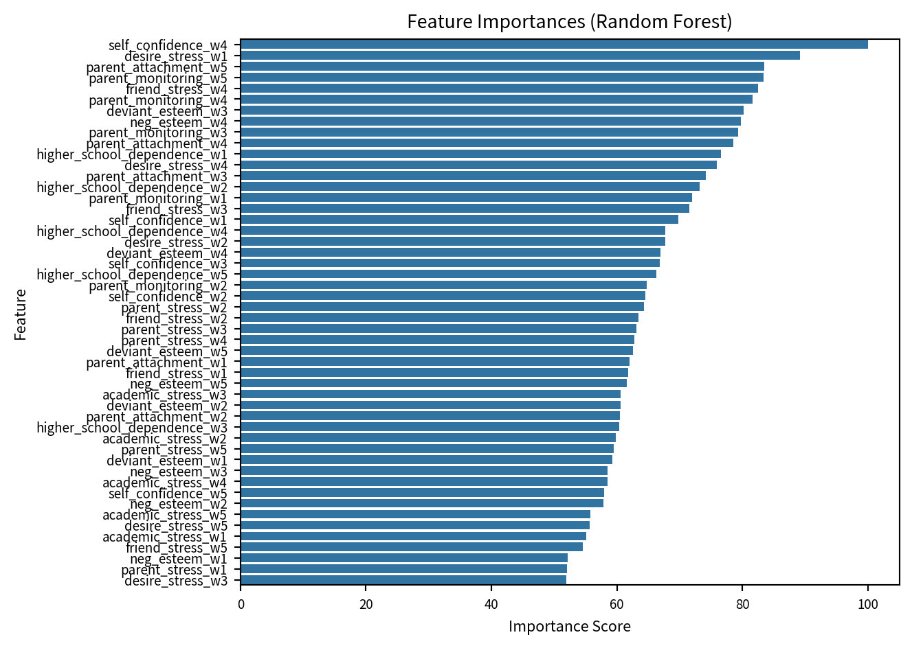
=== Random Forest 혼동 행렬 ===

                     Predicted: explorative  Predicted: stable
Actual: explorative                37334.03           44905.28
Actual: stable                     27479.79           63292.70

=== Random Forest 성능 지표 ===

정확도: 0.5816

Random Forest 범주별 정밀도:
explorative    0.576
stable         0.585
dtype: float64

Random Forest 범주별 재현율:
explorative    0.4540
stable         0.6973
dtype: float64

Random Forest 범주별 F1-score:
explorative    0.5078
stable         0.6362
dtype: float64
XGBoost
import xgboost as xgb
from sklearn.preprocessing import LabelEncoder

le = LabelEncoder()
y_train_numeric = le.fit_transform(y_train)
y_test_numeric = le.transform(y_test)

class_labels_ordered = list(le.classes_)
num_classes = len(class_labels_ordered)

print(f"Label Encoder 클래스: {class_labels_ordered} -> {list(range(num_classes))}")

xgb_model = xgb.XGBClassifier(
    objective='multi:softprob',
    eval_metric='mlogloss',
    num_class=num_classes,
    seed=RANDOM_STATE,
    use_label_encoder=False,
    verbosity=0
)

param_grid = {
    'n_estimators': [100, 200],
    'max_depth': [3, 5, 10, None],
    'learning_rate': [0.05, 0.1],
    'subsample': [0.8, 1.0],
    'colsample_bytree': [0.8, 1.0]
}

grid_search = GridSearchCV(
    estimator=xgb_model,
    param_grid=param_grid,
    cv=3,
    scoring='accuracy',
    n_jobs=-1,
    verbose=1
)

grid_search.fit(X_train, y_train_numeric, sample_weight=weights_train)

print(f"\n최적의 하이퍼파라미터: {grid_search.best_params_}")
print(f"최적 교차 검증 점수: {grid_search.best_score_:.4f}")

xgb_model_py = grid_search.best_estimator_

importance_scores = xgb_model_py.feature_importances_
xgb_importance_df = pd.DataFrame({
    'Feature': X_train.columns,
    'Importance': importance_scores
})

max_importance = xgb_importance_df['Importance'].max()
xgb_importance_df['Importance'] = (xgb_importance_df['Importance'] / max_importance) * 100
xgb_importance_df = xgb_importance_df.sort_values(by='Importance', ascending=False)

print("\nXGBoost 변수 중요도")
print(xgb_importance_df)

sns.barplot(x='Importance', y='Feature', data=xgb_importance_df)
plt.title('Feature Importances (XGBoost)', fontsize=10)
plt.xlabel('Importance', fontsize=8)
plt.ylabel('Feature', fontsize=8)
plt.xticks(fontsize=7)
plt.yticks(fontsize=7)
plt.tight_layout()
plt.savefig('xg_imp.png', dpi=300, bbox_inches='tight')
plt.show()

y_pred_proba_xgb = xgb_model_py.predict_proba(X_test)
y_pred_xgb_numeric = np.argmax(y_pred_proba_xgb, axis=1)
y_pred_xgb = le.inverse_transform(y_pred_xgb_numeric)
y_pred_xgb_cat = pd.Categorical(y_pred_xgb, categories=class_labels_ordered, ordered=False)

cm_xgb = confusion_matrix(y_test, y_pred_xgb_cat, sample_weight=weights_test, labels=class_labels_ordered)
print("\n=== XGBoost 모델 혼동 행렬 ===\n")
cm_df_xgb = pd.DataFrame(cm_xgb, index=[f"Actual: {cat}" for cat in class_labels_ordered], columns=[f"Predicted: {cat}" for cat in class_labels_ordered])
print(cm_df_xgb.round(2))

accuracy_xgb = accuracy_score(y_test, y_pred_xgb_cat, sample_weight=weights_test)
precision_xgb_sk = precision_score(y_test, y_pred_xgb_cat, sample_weight=weights_test, average=None, labels=class_labels_ordered, zero_division=0)
recall_xgb_sk = recall_score(y_test, y_pred_xgb_cat, sample_weight=weights_test, average=None, labels=class_labels_ordered, zero_division=0)
f1_score_xgb_sk = f1_score(y_test, y_pred_xgb_cat, sample_weight=weights_test, average=None, labels=class_labels_ordered, zero_division=0)

print("\n=== XGBoost 모델 성능 지표 ===\n")
print(f"정확도: {accuracy_xgb:.4f}")
print("\nXGBoost 모델 범주별 정밀도:")
print(pd.Series(precision_xgb_sk, index=class_labels_ordered).round(4))
print("\nXGBoost 모델 범주별 재현율:")
print(pd.Series(recall_xgb_sk, index=class_labels_ordered).round(4))
print("\nXGBoost 모델 범주별 F1-score:")
print(pd.Series(f1_score_xgb_sk, index=class_labels_ordered).round(4))
Label Encoder 클래스: ['explorative', 'stable'] -> [0, 1]
Fitting 3 folds for each of 64 candidates, totalling 192 fits
최적의 하이퍼파라미터: {'colsample_bytree': 0.8, 'learning_rate': 0.05, 'max_depth': 3, 'n_estimators': 100, 'subsample': 0.8}
최적 교차 검증 점수: nan
XGBoost 변수 중요도
Feature Importance
40 parent_attachment_w5 100.000000
38 neg_esteem_w4 89.684937
36 self_confidence_w4 87.710533
33 parent_monitoring_w4 84.155891
30 parent_attachment_w4 83.655487
35 friend_stress_w4 83.593765
23 parent_monitoring_w3 80.530685
15 friend_stress_w2 80.180794
12 parent_stress_w2 80.104950
6 self_confidence_w1 78.258446
17 higher_school_dependence_w2 77.525246
21 deviant_esteem_w3 75.736404
22 parent_stress_w3 74.421280
4 desire_stress_w1 74.244553
43 parent_monitoring_w5 74.036301
14 desire_stress_w2 73.580856
7 higher_school_dependence_w1 73.197128
25 friend_stress_w3 72.865379
47 higher_school_dependence_w5 72.309631
31 deviant_esteem_w4 71.178528
39 academic_stress_w4 69.950974
48 neg_esteem_w5 69.804626
32 parent_stress_w4 69.397591
3 parent_monitoring_w1 68.932785
46 self_confidence_w5 68.488029
45 friend_stress_w5 68.380692
26 self_confidence_w3 67.708191
27 higher_school_dependence_w3 66.273537
19 academic_stress_w2 65.726303
41 deviant_esteem_w5 65.552612
20 parent_attachment_w3 65.515610
11 deviant_esteem_w2 65.489426
9 academic_stress_w1 64.981789
34 desire_stress_w4 63.373531
49 academic_stress_w5 63.285591
42 parent_stress_w5 62.527847
13 parent_monitoring_w2 62.383938
24 desire_stress_w3 62.092834
18 neg_esteem_w2 61.555267
29 academic_stress_w3 60.970982
37 higher_school_dependence_w4 60.602821
44 desire_stress_w5 59.860622
5 friend_stress_w1 59.424625
0 parent_attachment_w1 55.924370
10 parent_attachment_w2 55.653919
8 neg_esteem_w1 52.370869
28 neg_esteem_w3 50.224579
2 parent_stress_w1 50.090385
1 deviant_esteem_w1 49.659233
16 self_confidence_w2 49.203815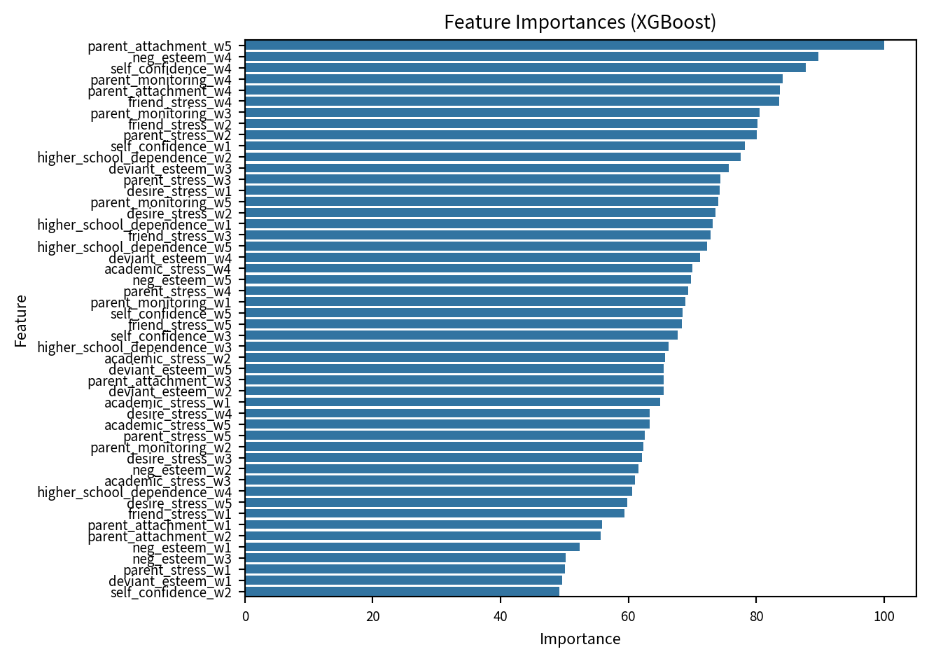
=== XGBoost 모델 혼동 행렬 ===

                     Predicted: explorative  Predicted: stable
Actual: explorative                40510.53           41728.78
Actual: stable                     25198.53           65573.96

=== XGBoost 모델 성능 지표 ===

정확도: 0.6132

XGBoost 모델 범주별 정밀도:
explorative    0.6165
stable         0.6111
dtype: float64

XGBoost 모델 범주별 재현율:
explorative    0.4926
stable         0.7224
dtype: float64

XGBoost 모델 범주별 F1-score:
explorative    0.5476
stable         0.6621
dtype: float64
Logistic Regression
from sklearn.linear_model import LogisticRegression
import statsmodels.api as sm

base_log_reg = LogisticRegression(
    solver='lbfgs',
    max_iter=5000,
    random_state=RANDOM_STATE,
    n_jobs=-1
)

param_grid = [
    {
        'penalty': ['l1'],
        'C': [0.001, 0.01, 0.1, 1, 10],
        'solver': ['liblinear', 'saga'],
        'class_weight': ['balanced', None]
    },
    {
        'penalty': ['l2'],
        'C': [0.001, 0.01, 0.1, 1, 10],
        'solver': ['lbfgs', 'liblinear', 'saga'],
        'class_weight': ['balanced', None]
    },
    {
        'penalty': ['elasticnet'],
        'C': [0.001, 0.01, 0.1, 1, 10],
        'solver': ['saga'],
        'l1_ratio': [0.2, 0.5, 0.8],
        'class_weight': ['balanced', None]
    }
]

grid_search = GridSearchCV(
    estimator=base_log_reg,
    param_grid=param_grid,
    cv=3,
    scoring='accuracy',
    n_jobs=-1,
    verbose=False
)

grid_search.fit(X_train, y_train, sample_weight=weights_train)

print(f"\n최적의 하이퍼파라미터: {grid_search.best_params_}")
print(f"최적 교차 검증 점수: {grid_search.best_score_:.4f}")

log_reg_model_py = grid_search.best_estimator_
class_labels_logreg = log_reg_model_py.classes_
coef_series = pd.Series(log_reg_model_py.coef_[0], index=X_train.columns)
sorted_coefs = coef_series.reindex(coef_series.abs().sort_values(ascending=False).index)

X_train_sm = sm.add_constant(X_train)
X_test_sm = sm.add_constant(X_test)

y_train_binary = (y_train == class_labels_logreg[1]).astype(int)

logit_model = sm.Logit(y_train_binary, X_train_sm)
logit_result = logit_model.fit(disp=0)

coef_summary = logit_result.summary2().tables[1]
coef_summary_df = pd.DataFrame(coef_summary)
coef_summary_sorted = coef_summary_df.sort_values('Coef.', key=abs, ascending=False)
print("\n계수 및 p-value (절댓값이 큰 순서):")
print(coef_summary_sorted[['Coef.', 'P>|z|']])

y_pred_logistic_py = log_reg_model_py.predict(X_test)

test_categories_logreg = list(y_test.cat.categories) if hasattr(y_test, 'cat') else sorted(list(y_test.unique()))
y_pred_logistic_cat = pd.Categorical(y_pred_logistic_py, categories=test_categories_logreg, ordered=False)

cm_logistic = confusion_matrix(y_test, y_pred_logistic_cat, sample_weight=weights_test, labels=test_categories_logreg)
print("\n=== 로지스틱 회귀 모델 혼동 행렬 ===\n")
cm_df_logistic = pd.DataFrame(cm_logistic, index=[f"Actual: {cat}" for cat in test_categories_logreg], columns=[f"Predicted: {cat}" for cat in test_categories_logreg])
print(cm_df_logistic.round(2))

accuracy_logistic = accuracy_score(y_test, y_pred_logistic_cat, sample_weight=weights_test)
precision_logistic_sk = precision_score(y_test, y_pred_logistic_cat, sample_weight=weights_test, average=None, labels=test_categories_logreg, zero_division=0)
recall_logistic_sk = recall_score(y_test, y_pred_logistic_cat, sample_weight=weights_test, average=None, labels=test_categories_logreg, zero_division=0)
f1_score_logistic_sk = f1_score(y_test, y_pred_logistic_cat, sample_weight=weights_test, average=None, labels=test_categories_logreg, zero_division=0)

print("\n=== 로지스틱 회귀 모델 성능 지표 ===\n")
print(f"정확도: {accuracy_logistic:.4f}")
print("\n로지스틱 회귀 모델 범주별 정밀도:")
print(pd.Series(precision_logistic_sk, index=test_categories_logreg).round(4))
print("\n로지스틱 회귀 모델 범주별 재현율:")
print(pd.Series(recall_logistic_sk, index=test_categories_logreg).round(4))
print("\n로지스틱 회귀 모델 범주별 F1-score:")
print(pd.Series(f1_score_logistic_sk, index=test_categories_logreg).round(4))
최적의 하이퍼파라미터: {'C': 0.1, 'class_weight': None, 'penalty': 'l2', 'solver': 'lbfgs'}
최적 교차 검증 점수: 0.6006

계수 및 p-value (절댓값이 큰 순서):
                                Coef.     P>|z|
desire_stress_w1             0.499608  0.000015
self_confidence_w4          -0.332916  0.010294
parent_stress_w3             0.271418  0.057369
neg_esteem_w4                0.263964  0.031803
desire_stress_w2             0.255400  0.018759
self_confidence_w3          -0.254064  0.030035
friend_stress_w4            -0.247249  0.024386
const                        0.245302  0.000002
deviant_esteem_w3           -0.237610  0.068700
parent_monitoring_w3         0.211999  0.050412
parent_attachment_w3         0.184476  0.274346
parent_monitoring_w4         0.180603  0.106346
higher_school_dependence_w5 -0.164889  0.024659
academic_stress_w2          -0.156225  0.223868
parent_attachment_w5         0.151586  0.345721
desire_stress_w3            -0.149660  0.181854
self_confidence_w2          -0.140414  0.185298
deviant_esteem_w1           -0.138070  0.263940
parent_stress_w4            -0.137391  0.383677
friend_stress_w1            -0.136979  0.134193
academic_stress_w5           0.118084  0.270881
parent_monitoring_w1         0.113677  0.264741
academic_stress_w1          -0.112715  0.410824
desire_stress_w4             0.110917  0.295629
self_confidence_w1           0.109299  0.356000
parent_stress_w1            -0.104439  0.436255
parent_stress_w2            -0.101390  0.460526
parent_monitoring_w2        -0.098915  0.363357
desire_stress_w5             0.096226  0.359037
neg_esteem_w1                0.096029  0.462255
academic_stress_w4           0.091028  0.451824
higher_school_dependence_w2 -0.086012  0.175999
higher_school_dependence_w1 -0.082377  0.182057
parent_attachment_w4        -0.078615  0.648722
deviant_esteem_w4           -0.077995  0.525561
neg_esteem_w5               -0.077245  0.532354
parent_monitoring_w5         0.075278  0.495239
friend_stress_w5            -0.073577  0.475849
friend_stress_w2            -0.069986  0.466378
higher_school_dependence_w4 -0.059155  0.445485
parent_stress_w5            -0.053443  0.710032
neg_esteem_w3               -0.045219  0.687428
parent_attachment_w1        -0.035101  0.822711
higher_school_dependence_w3  0.033887  0.623319
deviant_esteem_w5           -0.024602  0.843547
neg_esteem_w2                0.021549  0.824973
academic_stress_w3          -0.017071  0.879205
self_confidence_w5           0.015841  0.893445
friend_stress_w3            -0.010240  0.924892
parent_attachment_w2         0.006187  0.967933
deviant_esteem_w2            0.002349  0.982333

=== 로지스틱 회귀 모델 혼동 행렬 ===

                     Predicted: explorative  Predicted: stable
Actual: explorative                42190.16           40049.15
Actual: stable                     26537.42           64235.07

=== 로지스틱 회귀 모델 성능 지표 ===

정확도: 0.6151

로지스틱 회귀 모델 범주별 정밀도:
explorative    0.6139
stable         0.6160
dtype: float64

로지스틱 회귀 모델 범주별 재현율:
explorative    0.5130
stable         0.7076
dtype: float64

로지스틱 회귀 모델 범주별 F1-score:
explorative    0.5589
stable         0.6586
dtype: float64
모델 성능 비교
import matplotlib.cm as cm

model_metrics_list = []
class_labels_ordered = list(y_test.cat.categories)

def compile_metrics(model_name, accuracy, precision_arr, recall_arr, f1_arr):
    metrics = {'Model': model_name, 'Accuracy': accuracy}
    for i, label in enumerate(class_labels_ordered):
        metrics[f'Precision ({label})'] = precision_arr[i]
        metrics[f'Recall ({label})'] = recall_arr[i]
        metrics[f'F1-score ({label})'] = f1_arr[i]
    return metrics

model_metrics_list.append(compile_metrics(
    "Random Classifier",
    accuracy_random,
    precision_random_sk,
    recall_random_sk,
    f1_score_random_sk
))
model_metrics_list.append(compile_metrics(
    "Random Forest",
    accuracy_rf,
    precision_rf_sk,
    recall_rf_sk,
    f1_score_rf_sk
))
model_metrics_list.append(compile_metrics(
    "XGBoost",
    accuracy_xgb,
    precision_xgb_sk,
    recall_xgb_sk,
    f1_score_xgb_sk
))
model_metrics_list.append(compile_metrics(
    "Logistic Regression",
    accuracy_logistic,
    precision_logistic_sk,
    recall_logistic_sk,
    f1_score_logistic_sk
))

comparison_df = pd.DataFrame(model_metrics_list).set_index('Model')
models = comparison_df.index.tolist()
all_categories = ['Accuracy']
for label in class_labels_ordered:
    all_categories.extend([
        f'Precision ({label})',
        f'Recall ({label})',
        f'F1-score ({label})'
    ])
angles = np.linspace(0, 2*np.pi, len(all_categories), endpoint=False).tolist()
angles += angles[:1]
ax = plt.subplot(111, polar=True)
colors = cm.tab10(np.linspace(0, 1, len(models)))
for i, model in enumerate(models):
    values = comparison_df.loc[model, all_categories].values.flatten().tolist()
    values += values[:1]
    ax.plot(angles, values, 'o-', linewidth=2, color=colors[i], label=model, alpha=0.8)
    ax.fill(angles, values, color=colors[i], alpha=0.1)
ax.set_xticks(angles[:-1])
ax.set_xticklabels(all_categories, fontsize=10)

ax.set_ylim(0, 1)
ax.set_yticks([0.2, 0.4, 0.6, 0.8, 1.0])
ax.set_yticklabels(['0.2', '0.4', '0.6', '0.8', '1.0'], fontsize=9)
ax.grid(True, linestyle='-', alpha=0.3)
plt.title('모델 성능 비교', size=15, y=1.1)
plt.legend(loc='upper right', bbox_to_anchor=(0.1, 0.1))
plt.savefig('model_met.png', dpi=300, bbox_inches='tight')
plt.tight_layout()
plt.show()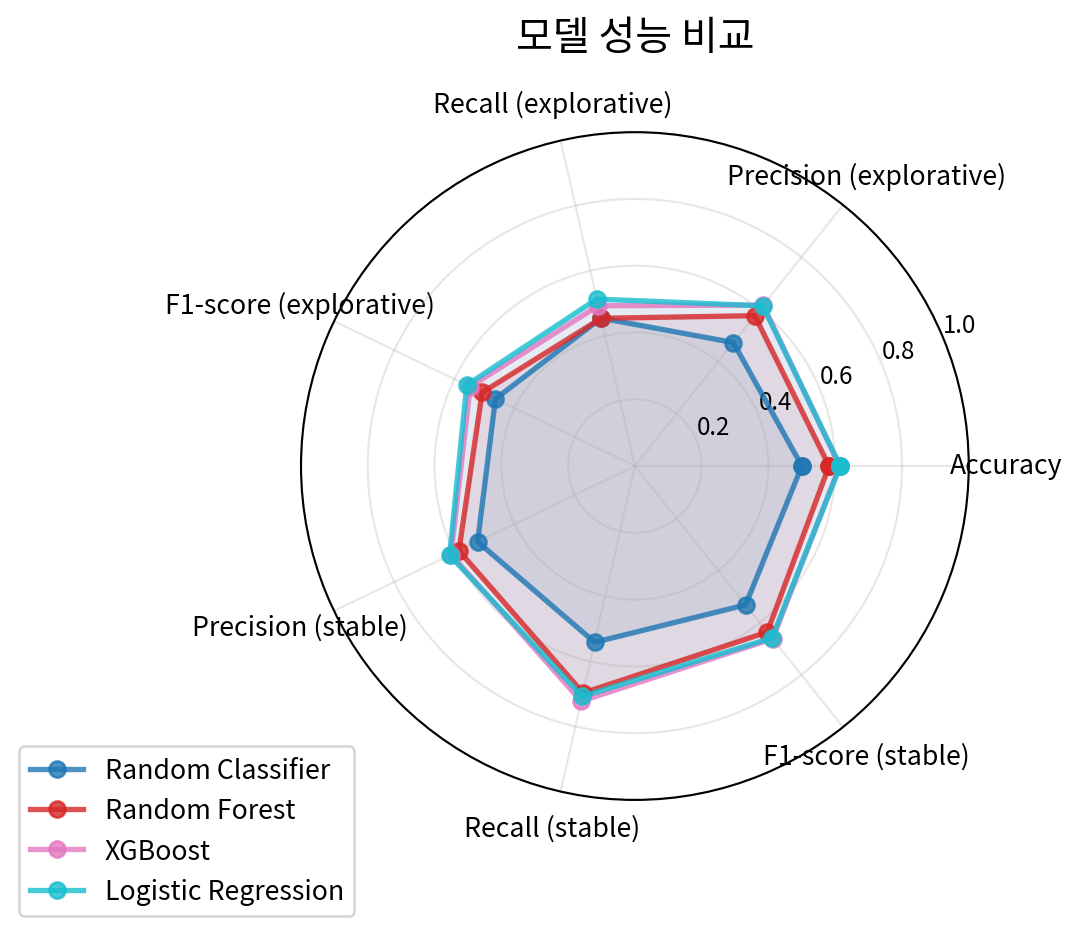
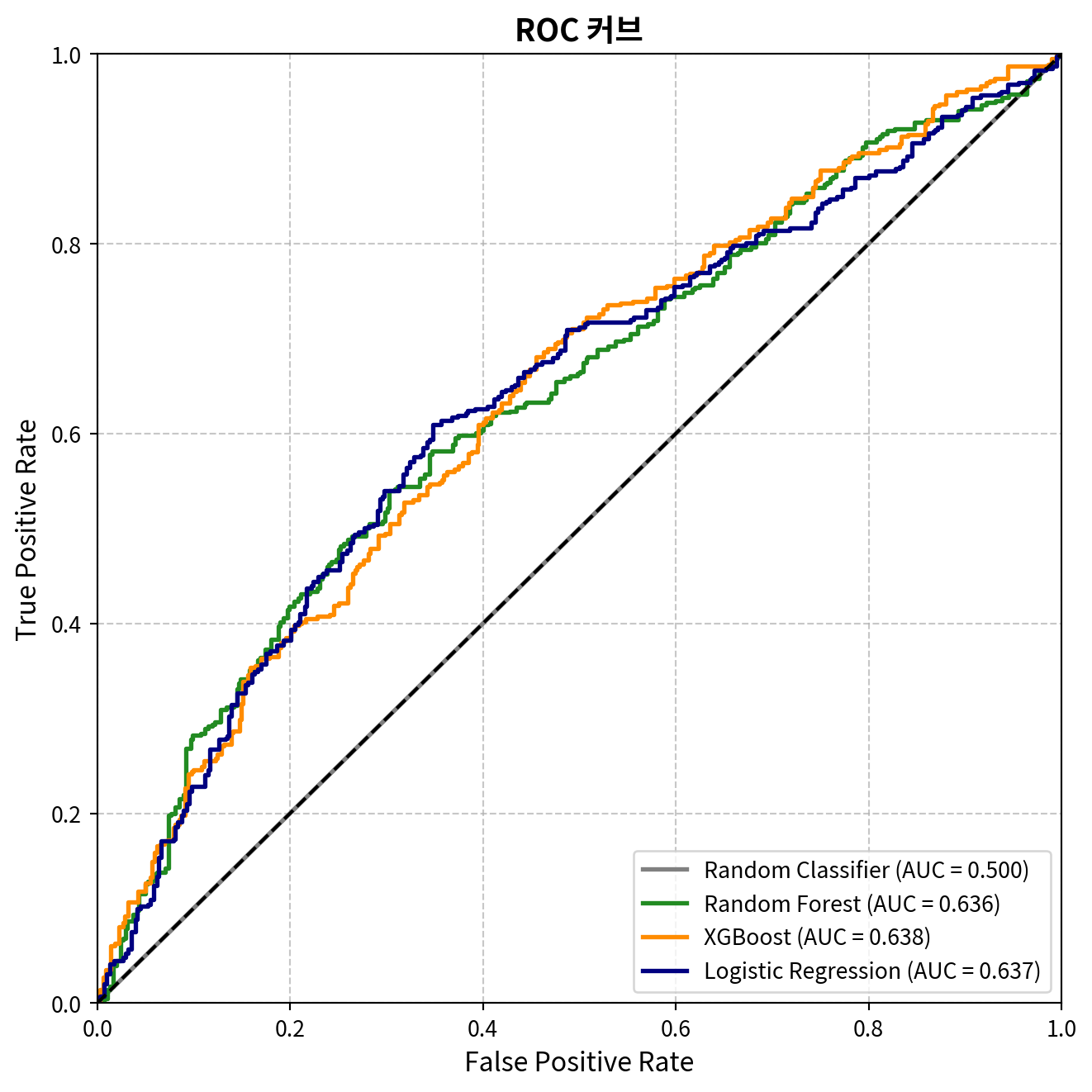
ROC 커브
random_pred_proba = np.zeros((len(y_test), len(class_labels_ordered)))
for i, cls in enumerate(class_labels_ordered):
    random_pred_proba[:, i] = prop_values_ordered[i]

pred_probas = {
    "Random Classifier": random_pred_proba,
    "Random Forest": y_pred_proba_rf,
    "XGBoost": y_pred_proba_xgb,
    "Logistic Regression": log_reg_model_py.predict_proba(X_test)
}

colors = {
    "Random Classifier": "grey",
    "Random Forest": "forestgreen",
    "XGBoost": "darkorange",
    "Logistic Regression": "navy"
}

y_test_numeric = y_test.cat.codes if hasattr(y_test, 'cat') else y_test

for model_name, proba in pred_probas.items():
    if proba.shape[1] > 1:
        y_score = proba[:, 1]
    else:
        y_score = proba.ravel()
    fpr, tpr, _ = roc_curve(y_test_numeric, y_score, sample_weight=weights_test)
    roc_auc = auc(fpr, tpr)
    plt.plot(fpr, tpr, lw=2, label=f'{model_name} (AUC = {roc_auc:.3f})', color=colors[model_name])

plt.plot([0, 1], [0, 1], 'k--', lw=1.5)
plt.xlim([0.0, 1.0])
plt.ylim([0.0, 1.0])
plt.xlabel('False Positive Rate', fontsize=12)
plt.ylabel('True Positive Rate', fontsize=12)
plt.title('ROC 커브', fontsize=14, fontweight='bold')
plt.legend(loc="lower right", fontsize=10)
plt.grid(True, linestyle='--', alpha=0.7)
plt.gcf().set_size_inches(7, 7)
plt.tight_layout()
plt.savefig('roc_curve_comparison.png', dpi=300, bbox_inches='tight')
plt.show()