from sklearn.tree import DecisionTreeClassifier, export_graphviz
from sklearn.datasets import load_iris
from sklearn.model_selection import train_test_split
import graphviz
import warnings

warnings.filterwarnings('ignore')분류 - 결정 트리
머신 러닝

개요
- 결정 노드가 많아지면 과적합이 발생할 수 있음
- 가능한 한 적은 결정 노드로 높은 예측 정확도를 가지려면 데이터를 분류할 때 최대한 많은 데이터 세트가 해당 분류에 속할 수 있도록 규칙을 정해야 함
- 균일하게 데이터 세트를 구성할 수 있도록 분할하는 것이 필요
- 균일도만 신경쓰면 되기 때문에 전처리 작업이 필요 없음
파라미터
- min_samples_split: 노드를 분할하기 위한 최소한의 샘플 수.
- min_samples_leaf: 말단 노드가 되기 위한 최소한의 샘플 수. 비대칭적 데이터의 경우 특정 클래스의 데이터가 극도로 작을 수 있으므로 작게 설정 필요
- max_features: 분할을 고려할 feature의 수. default는 None으로 모든 feature를 고려함
- max_depth
- max_leaf_nodes
시각화
dt_clf = DecisionTreeClassifier()

iris_data = load_iris()
X_train, X_test, y_train, y_test = train_test_split(iris_data.data, iris_data.target, test_size=0.2)

dt_clf.fit(X_train, y_train)DecisionTreeClassifier()In a Jupyter environment, please rerun this cell to show the HTML representation or trust the notebook.
On GitHub, the HTML representation is unable to render, please try loading this page with nbviewer.org.
DecisionTreeClassifier()
export_graphviz(dt_clf, out_file="tree.dot", class_names=iris_data.target_names, feature_names=iris_data.feature_names, impurity=True, filled=True)
with open("tree.dot") as f:
    dot_graph = f.read()
graphviz.Source(dot_graph)
import seaborn as sns
import numpy as np

for name, value in zip(iris_data.feature_names, dt_clf.feature_importances_):
    print(f'{name}: {value:.3f}')
sns.barplot(x=dt_clf.feature_importances_, y=iris_data.feature_names)
sepal length (cm): 0.043
sepal width (cm): 0.030
petal length (cm): 0.903
petal width (cm): 0.024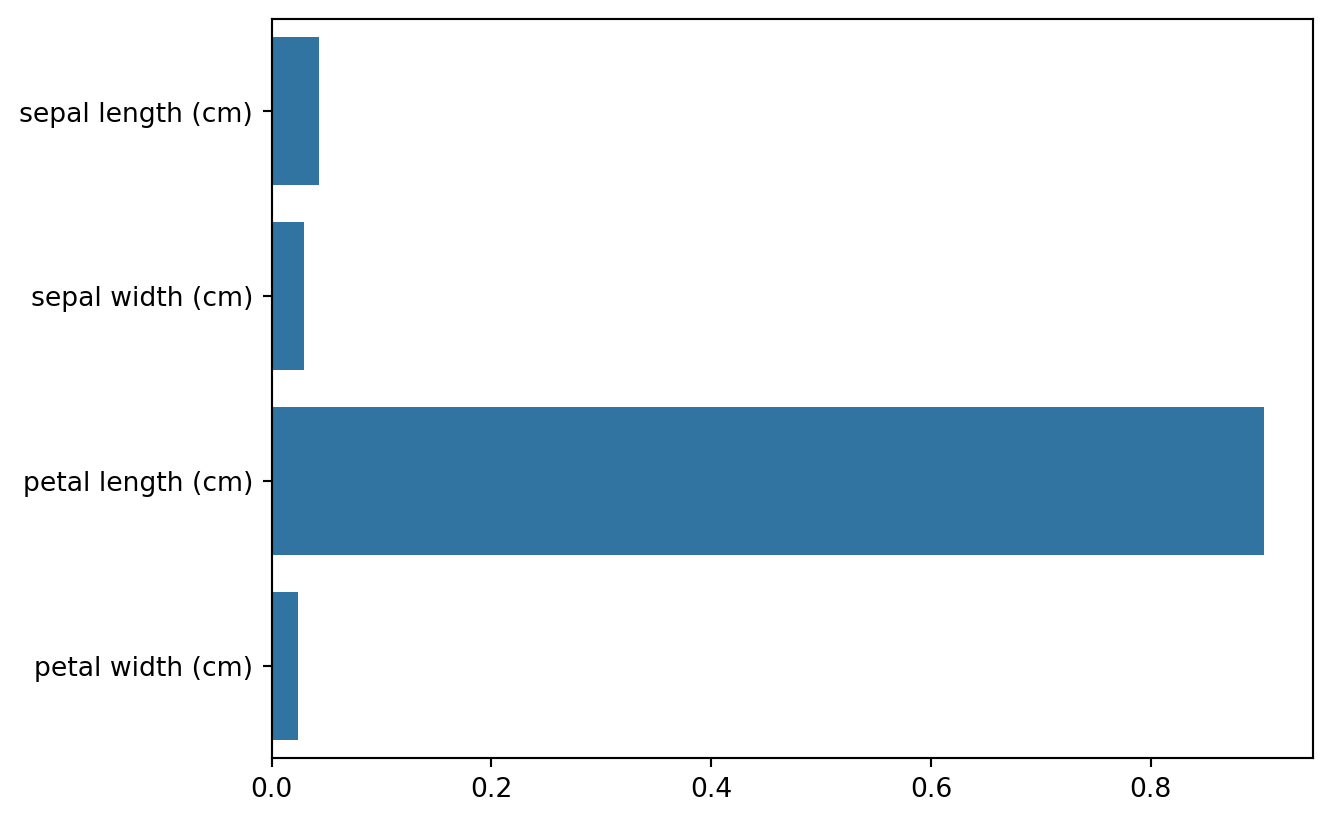
examples
import pandas as pd


def get_new_feature_name_df(old):
    df = pd.DataFrame(data=old.groupby('column_name').cumcount(), columns=['dup_cnt'])
    df = df.reset_index()
    new_df = pd.merge(old.reset_index(), df, how='outer')
    new_df['column_name'] = new_df[['column_name', 'dup_cnt']].apply(lambda x: x[0] + '_' + str(x[1]) if x[1] > 0 else x[0], axis=1)
    new_df = new_df.drop(['index'], axis=1)
    return new_df

def get_human_dataset():
    feature_name_df = pd.read_csv('_data/human_activity/features.txt', sep='\s+', header=None, names=['column_index', 'column_name'])
    new_feature_name_df = get_new_feature_name_df(feature_name_df)
    feature_name = new_feature_name_df.iloc[:, 1].values.tolist()

    X_train = pd.read_csv('_data/human_activity/train/X_train.txt', sep='\s+', names=feature_name)
    X_test = pd.read_csv('_data/human_activity/test/X_test.txt', sep='\s+', names=feature_name)

    y_train = pd.read_csv('_data/human_activity/train/y_train.txt', sep='\s+', header=None, names=['action'])
    y_test = pd.read_csv('_data/human_activity/test/y_test.txt', sep='\s+', header=None, names=['action'])

    return X_train, X_test, y_train, y_test

X_train, X_test, y_train, y_test = get_human_dataset()
X_train.info()
<class 'pandas.core.frame.DataFrame'>
RangeIndex: 7352 entries, 0 to 7351
Columns: 561 entries, tBodyAcc-mean()-X to angle(Z,gravityMean)
dtypes: float64(561)
memory usage: 31.5 MBy_train['action'].value_counts()action
6 1407
5 1374
4 1286
1 1226
2 1073
3 986
Name: count, dtype: int64default 파라미터 예측
from sklearn.metrics import accuracy_score

dt_clf = DecisionTreeClassifier()
dt_clf.fit(X_train, y_train)
pred = dt_clf.predict(X_test)
accuracy = accuracy_score(y_test, pred)
accuracy0.8551068883610451하이퍼파라미터 최적화
from sklearn.model_selection import GridSearchCV

params = {
    'max_depth': [6, 8, 10, 12, 16, 20, 24],
    'min_samples_split': [16]
}

grid_cv = GridSearchCV(dt_clf, param_grid=params, scoring='accuracy',cv=5, verbose=1)
grid_cv.fit(X_train, y_train)

cv_results_df = pd.DataFrame(grid_cv.cv_results_)
cv_results_df[['param_max_depth', 'mean_test_score']]
cv_results_df
Fitting 5 folds for each of 7 candidates, totalling 35 fits| mean_fit_time | std_fit_time | mean_score_time | std_score_time | param_max_depth | param_min_samples_split | params | split0_test_score | split1_test_score | split2_test_score | split3_test_score | split4_test_score | mean_test_score | std_test_score | rank_test_score | |
|---|---|---|---|---|---|---|---|---|---|---|---|---|---|---|---|
| 0 | 1.594731 | 0.052014 | 0.004070 | 0.000165 | 6 | 16 | {'max_depth': 6, 'min_samples_split': 16} | 0.808973 | 0.870836 | 0.814286 | 0.873469 | 0.870068 | 0.847527 | 0.029380 | 3 |
| 1 | 2.000555 | 0.035501 | 0.004050 | 0.000222 | 8 | 16 | {'max_depth': 8, 'min_samples_split': 16} | 0.802175 | 0.828688 | 0.859184 | 0.877551 | 0.891156 | 0.851751 | 0.032445 | 2 |
| 2 | 2.510755 | 0.267397 | 0.004037 | 0.000161 | 10 | 16 | {'max_depth': 10, 'min_samples_split': 16} | 0.815772 | 0.819171 | 0.847619 | 0.887755 | 0.904762 | 0.855016 | 0.035850 | 1 |
| 3 | 2.708626 | 0.200801 | 0.003862 | 0.000161 | 12 | 16 | {'max_depth': 12, 'min_samples_split': 16} | 0.791978 | 0.821890 | 0.852381 | 0.889116 | 0.880272 | 0.847127 | 0.036242 | 4 |
| 4 | 3.054742 | 0.530318 | 0.004009 | 0.000171 | 16 | 16 | {'max_depth': 16, 'min_samples_split': 16} | 0.802175 | 0.815092 | 0.834014 | 0.890476 | 0.882313 | 0.844814 | 0.035523 | 5 |
| 5 | 2.892980 | 0.253108 | 0.004152 | 0.000542 | 20 | 16 | {'max_depth': 20, 'min_samples_split': 16} | 0.797417 | 0.815772 | 0.842177 | 0.876190 | 0.878912 | 0.842093 | 0.032271 | 7 |
| 6 | 2.908142 | 0.248562 | 0.003913 | 0.000084 | 24 | 16 | {'max_depth': 24, 'min_samples_split': 16} | 0.808294 | 0.817811 | 0.831293 | 0.878912 | 0.883673 | 0.843996 | 0.031353 | 6 |
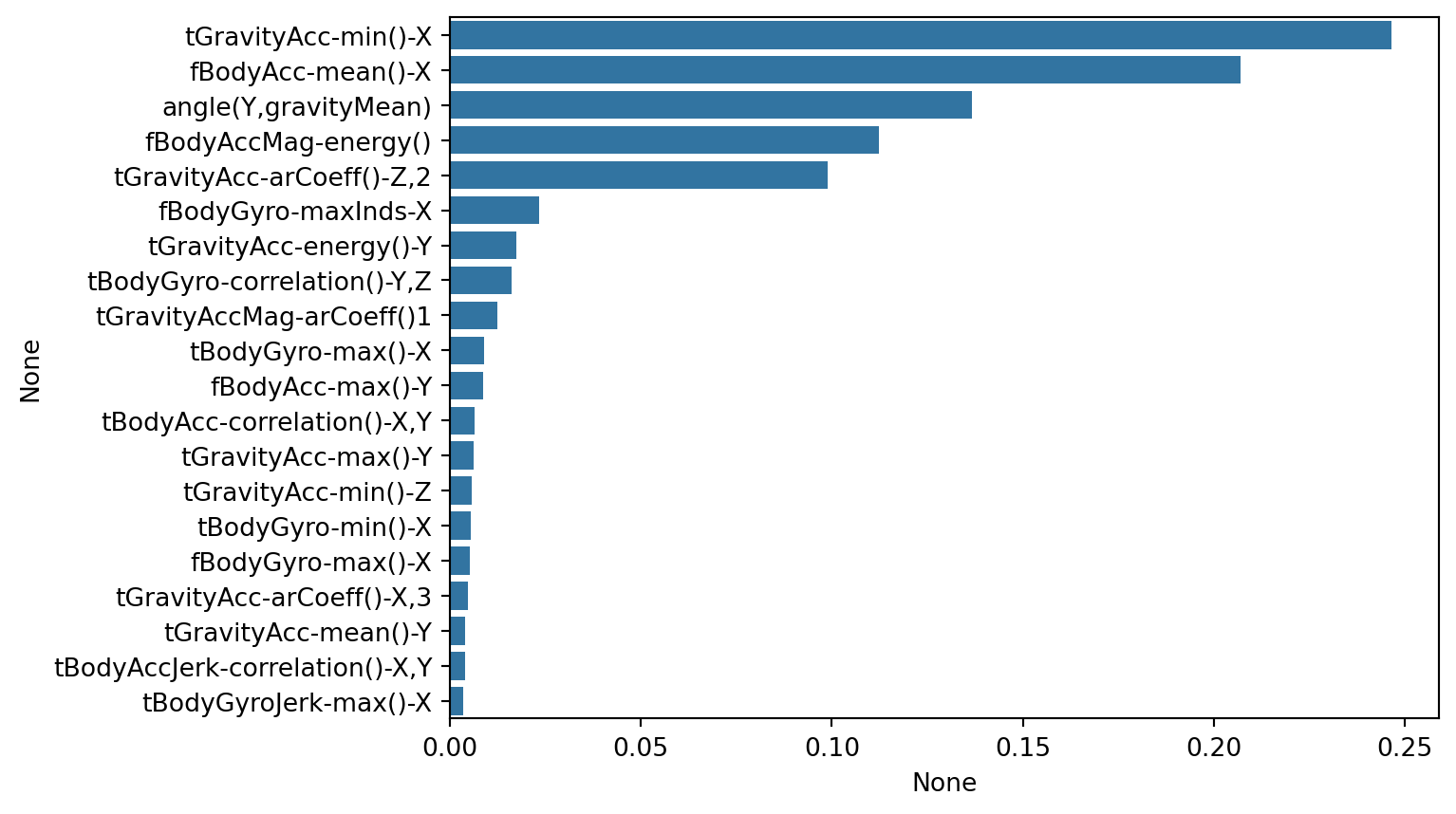
best_df_clf = grid_cv.best_estimator_

ftr_importances_values = best_df_clf.feature_importances_
ftr_importances = pd.Series(ftr_importances_values, index=X_train.columns)
ftr_top20 = ftr_importances.sort_values(ascending=False)[:20]
sns.barplot(x=ftr_top20, y=ftr_top20.index)