import numpy as np
import matplotlib.pyplot as plt

X = 2 * np.random.rand(100, 1)
y = 6 + 4 * X + np.random.randn(100, 1)
plt.scatter(X, y)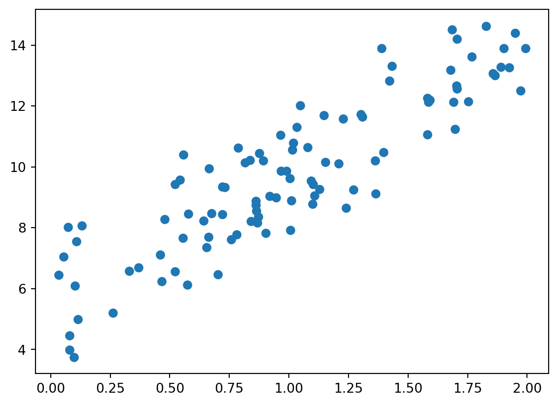

import numpy as np
import matplotlib.pyplot as plt
X = 2 * np.random.rand(100, 1)
y = 6 + 4 * X + np.random.randn(100, 1)
plt.scatter(X, y)
def get_cost(y, y_pred):
    N = len(y)
    cost = np.sum(np.square(y - y_pred)) / N
    return cost

def get_weight_updates(w1, w0, X, y, learning_rate=0.01):
    N = len(y)
    w1_update = np.zeros_like(w1)
    w0_update = np.zeros_like(w0)
    y_pred = np.dot(X, w1.T) + w0
    diff = y - y_pred

    w1_update = -(2/N) * learning_rate * np.dot(X.T, diff)
    w0_update = -(2/N) * learning_rate * np.sum(diff)

    return w1_update, w0_update

def gradient_descent_steps(X, y, iters=10000):
    w0 = np.zeros((1, 1))
    w1 = np.zeros((1, 1))

    for _ in range(iters):
        w1_update, w0_update = get_weight_updates(w1, w0, X, y, learning_rate=0.01)
        w1 = w1 - w1_update
        w0 = w0 - w0_update

    return w1, w0
w1, w0 = gradient_descent_steps(X, y, iters=1000)
y_pred = w1[0, 0] * X + w0
print(f'w0: {w0[0, 0]:.3f} w1: {w1[0, 0]:.3f}, total cost: {get_cost(y, y_pred):.3f}')
plt.scatter(X, y)
plt.plot(X, y_pred)w0: 5.452 w1: 4.276, total cost: 1.360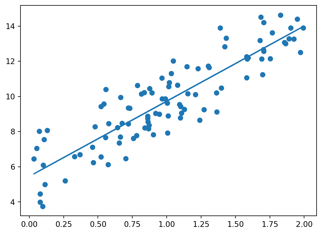
def stochastic_gradient_descent_steps(X, y, batch_size=10, iters=1000):
    w0 = np.zeros((1, 1))
    w1 = np.zeros((1, 1))

    for ind in range(iters):
        stochastic_random_index = np.random.permutation(X.shape[0])
        sample_X = X[stochastic_random_index[0:batch_size]]
        sample_y = y[stochastic_random_index[0:batch_size]]

        w1_update, w0_update = get_weight_updates(w1, w0, sample_X, sample_y, learning_rate=0.01)
        w1 = w1 - w1_update
        w0 = w0 - w0_update

    return w1, w0
w1, w0 = stochastic_gradient_descent_steps(X, y, iters=1000)
y_pred = w1[0, 0] * X + w0
print(f'w0: {w0[0, 0]:.3f} w1: {w1[0, 0]:.3f}, total cost: {get_cost(y, y_pred):.3f}')
plt.scatter(X, y)
plt.plot(X, y_pred)w0: 5.464 w1: 4.263, total cost: 1.360
import pandas as pd
import seaborn as sns
from scipy import stats
from sklearn.datasets import load_boston
import warnings

warnings.filterwarnings('ignore')

boston = load_boston()

df = pd.DataFrame(boston.data, columns=boston.feature_names)
df['price'] = boston.target
df.head()
lm_features = ['RM', 'ZN', 'INDUS', 'NOX', 'AGE', 'PTRAIO', 'LSTAT', 'RAD']
fig, axs = plt.subplots(figsize=(16, 8), ncols=len(lm_features) // 2, nrows=2)
for i, feature in enumerate(lm_features):
row = i // 4
col = i % 4
sns.regplot(x=feature, y='price', data=df, ax=axs[row][col])boston 데이터가 윤리적 문제로 사용 불가능하다고 한다.
from sklearn.linear_model import LinearRegression
from sklearn.model_selection import cross_val_score

y_target = df['price']
X_data = df.drop(['price'], axis=1, inplace=False)
lr = LinearRegression()

neg_mse_scores = cross_val_score(lr, X_data, y_target, scoring="neg_mean_squared_error", cv=5)
rmse_scores = np.sqrt(-1 * neg_mse_scores)
avg_rmse = np.mean(rmse_scores)
cross_val_score는 값이 큰걸 좋게 평가해서 neg를 기준으로 넣어줘야함
from sklearn.preprocessing import PolynomialFeatures
from sklearn.linear_model import LinearRegression
from sklearn.pipeline import Pipeline

def polynominal_func(X):
    y = 1 + 2 * X[:, 0] + 3 * X[:, 0]**2 + 4 * X[:, 1]**3
    return y

model = Pipeline([('poly', PolynomialFeatures(degree=3)),
                  ('linear', LinearRegression())])
X = np.arange(4).reshape(2, 2)
y = polynominal_func(X)

model = model.fit(X, y)

np.round(model.named_steps['linear'].coef_, 2)
array([0. , 0.18, 0.18, 0.36, 0.54, 0.72, 0.72, 1.08, 1.62, 2.34])L2 규제(Ridge): \(min(RSS(W) + \lambda ||W||^2)\)
L1 규제(Lasso): \(min(RSS(W) + \lambda ||W||_1)\)
λ가 크면, 회귀계수의 크기가 작아지고, λ가 0이 되면 일반 선형회귀와 같아짐
L1 규제는 영향력이 작은 피처의 계수를 0으로 만들어서 피처 선택 효과가 있음. L2는 0으로 만들지는 않음
from sklearn.linear_model import Ridge

ridge = Ridge(alpha = 10)
neg_mse_scores = cross_val_score(ridge, X_data, y_target, scoring="neg_mean_squared_error", cv=5)
rmse_scores = np.sqrt(-1 * neg_mse_scores)
avg_rmse = np.mean(rmse_scores)import pandas as pd
from sklearn.linear_model import Ridge, Lasso, ElasticNet
def get_linear_reg_eval(model_name, params=None, X_data_n=None, y_target_n=None):
coeff_df = pd.DataFrame()
for param in params:
if model_name == 'Ridge':
model = Ridge(alpha=param)
elif model_name == 'Lasso':
model = Lasso(alpha=param)
elif model_name == 'ElasticNet':
model = ElasticNet(alpha=param, l1_ratio=0.7)
neg_mse_scores = cross_val_score(model, X_data_n, y_target_n, scoring="neg_mean_squared_error", cv=5)
rmse_scores = np.sqrt(-1 * neg_mse_scores)
avg_rmse = np.mean(rmse_scores)
print(f'{param}: {avg_rmse:.3f}')
model.fit(X_data_n, y_target_n)
coeff = pd.Series(data=model.coef_, index=X_data_n.columns)
colname = 'alpha:' + str(param)
coeff_df[colname] = coeff
return coeff_dfnp.log1p(data)