import numpy as np
from empiricaldist import Pmf

hypos = np.arange(1, 1001)
prior = Pmf(1, hypos)수량 추정
확률 통계

기관차 문제
- 각 철도를 지나가는 기관차에 1부터 N까지의 순서로 번호를 붙인다.
- 60번 번호가 붙은 기관차를 보았다.
- 이 철도에 몇 개의 기관차가 지나가는지 추정해보자
- 가정: N은 1부터 1000까지의 값 중 한 값이 동일한 확률로 선택될 수 있다.
def update_train(pmf, data):
  hypos = pmf.qs
  likelihood = 1 / hypos
  likelihood[(data > hypos)] = 0
  pmf *= likelihood
  pmf.normalize()
data = 60
posterior = prior.copy()
update_train(posterior, data)import matplotlib.pyplot as plt
plt.rcParams['font.family'] = 'Noto Sans KR'
posterior.plot(label='60번 기관차 발견 시 전체 기관차 수의 사후확률', color='C5')
plt.legend()
plt.title('사후 확률')
plt.xlabel('기관차 수')
plt.ylabel('PMF')Text(0, 0.5, 'PMF')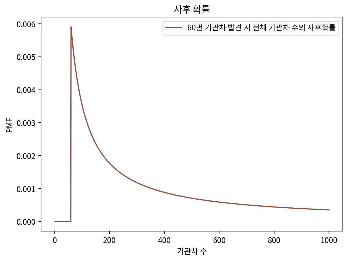
posterior.max_prob()60- 당연하다는 듯이 60이 최선의 선택. 하지만 이는 별로 도움이 안됨.
- 대안으로 사후확률의 평균을 구해본다.
posterior.mean()333.41989326370776- 해당 값을 선택하는 것이 장기적으로 좋은 선택.
import pandas as pd

df = pd.DataFrame(columns=['사후확률 분포 평균'])
df.index.name = '상한값'

dataset = [30, 60, 90]

for high in [500, 1000, 2000]:
    hypos = np.arange(1, high+1)
    pmf = Pmf(1, hypos)
    for data in dataset:
        update_train(pmf, data)
    df.loc[high] = pmf.mean()
df| 사후확률 분포 평균 | |
|---|---|
| 상한값 | |
| 500 | 151.849588 |
| 1000 | 164.305586 |
| 2000 | 171.338181 |
- 하지만 상한값의 범위의 변화에 따른 사후확률 분포의 평균값이 크게 달라진다.
- 이럴때는 2가지 방법이 있다.
- 데이터를 더 확보
- 배경지식을 더 확보해서 더 나은 사전확률을 선택
멱법칙 사전확률
- 기관차 수는 멱법칙을 주로 따르는 것으로 알려져 있음
- 더 적합한 사전확률은 안정적인 사전확률을 제공할 수 있다.
alpha = 1.0
ps = hypos ** (-alpha)
power = Pmf(ps, hypos, name='power law')
power.normalize()8.178368103610282uniform = Pmf(1, hypos, name='uniform')
uniform.normalize()
power.plot(label='power', color='skyblue')
uniform.plot(label='uniform', color='pink')
plt.legend()
plt.title('사전확률 분포')
plt.xlabel('기관차 수')
plt.ylabel('PMF')Text(0, 0.5, 'PMF')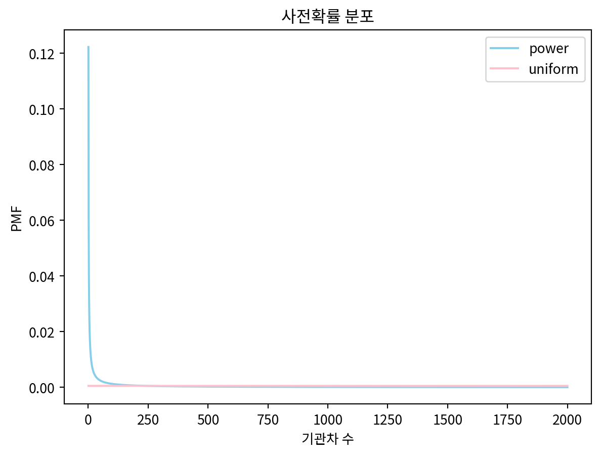
update_train(uniform, 60)
update_train(power, 60)

power.plot(label='power', color='skyblue')
uniform.plot(label='uniform', color='pink')
plt.legend()
plt.title('사후확률 분포')
plt.xlabel('기관차 수')
plt.ylabel('PMF')
Text(0, 0.5, 'PMF')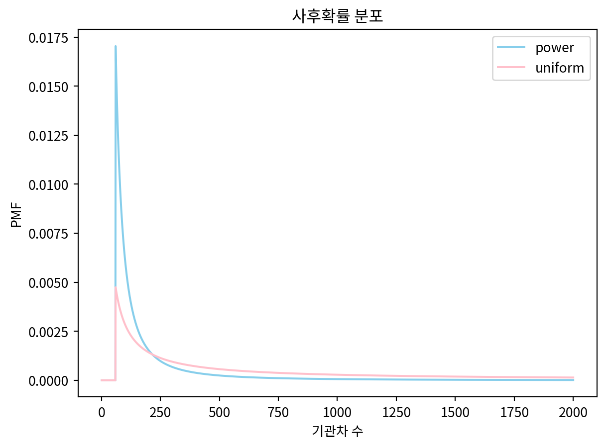
df = pd.DataFrame(columns=['사후확률 분포 평균'])
df.index.name = '상한값'

alpha = 1.0
dataset = [30, 60, 90]

for high in [500, 1000, 2000]:
    hypos = np.arange(1, high+1)
    ps = hypos**(-alpha)
    power = Pmf(ps, hypos)
    for data in dataset:
        update_train(power, data)
    df.loc[high] = power.mean()
df| 사후확률 분포 평균 | |
|---|---|
| 상한값 | |
| 500 | 130.708470 |
| 1000 | 133.275231 |
| 2000 | 133.997463 |
신뢰구간
power.credible_interval(0.9)array([ 91., 243.])연습문제
5-1
from scipy.stats import binom

def update(pmf, k, p):
    likelihood = binom.pmf(k, pmf.qs, p)
    pmf *= likelihood
    pmf.normalize()

hypos = np.arange(1, 2001)
prior = Pmf(1, hypos)

posterior = prior.copy()

update(posterior, 2, 1/365)
print(f"5월 11일 데이터 적용 후 평균 인원수: {posterior.mean():.1f}")

update(posterior, 1, 1/365)
print(f"5월 23일 데이터 적용 후 평균 인원수: {posterior.mean():.1f}")

update(posterior, 0, 1/365)
print(f"8월 1일 데이터 적용 후 평균 인원수: {posterior.mean():.1f}")
5월 11일 데이터 적용 후 평균 인원수: 957.1
5월 23일 데이터 적용 후 평균 인원수: 721.7
8월 1일 데이터 적용 후 평균 인원수: 486.2estimated_people = posterior.mean()
print(f"추정된 강당 인원수: {estimated_people:.1f}명")
prob_over_1200 = posterior[posterior.qs > 1200].sum()
print(f"1200명을 초과할 확률: {prob_over_1200:.4f} ({prob_over_1200*100:.2f}%)")
ci_90 = posterior.credible_interval(0.9)
print(f"90% 신뢰구간: [{ci_90[0]:.0f}, {ci_90[1]:.0f}]")추정된 강당 인원수: 486.2명
1200명을 초과할 확률: 0.0112 (1.12%)
90% 신뢰구간: [166, 942]5-2
def rabbit_likelihood(n):
    return ((n - 1) / n) * (1/n) * (1/n) * 3

hypos = np.arange(4, 11)
prior = Pmf(1, hypos)

likelihood = [rabbit_likelihood(n) for n in hypos]

posterior = prior.copy()
posterior *= likelihood
posterior.normalize()

print(f"\n추정 토끼 수 (평균): {posterior.mean():.2f}마리")
추정 토끼 수 (평균): 5.92마리5-3
def update_remain(pmf, data):
    hypos = pmf.qs
    likelihood = 1 / hypos
    likelihood[(hypos < data)] = 0
    pmf *= likelihood
    pmf.normalize()

hypos = np.arange(0, 1096)
prior = Pmf(1, hypos)
prior.normalize()

update_remain(prior, 1095)
prior.plot(label='사후확률', color='pink')
plt.legend()
plt.show()
5-5
import numpy as np
from empiricaldist import Pmf

hypos_short = np.arange(0, 201) # 10억 단위
prior_short = Pmf(1, hypos_short, name="short")
prior_short.normalize()

hypos_long = np.arange(0, 2001)
prior_long = Pmf(1, hypos_long, name="long")
prior_long.normalize()

likelihood_ps = {}
for pmf in [prior_short, prior_long]:
    likelihood = 1 / pmf.qs
    likelihood[(pmf.qs < 108)] = 0
    pmf *= likelihood
    pmf.normalize()
    likelihood_ps[pmf.name] = pmf(108)
    pmf.plot(label=f"{pmf.name}: {pmf(108)}")
plt.legend()
plt.show()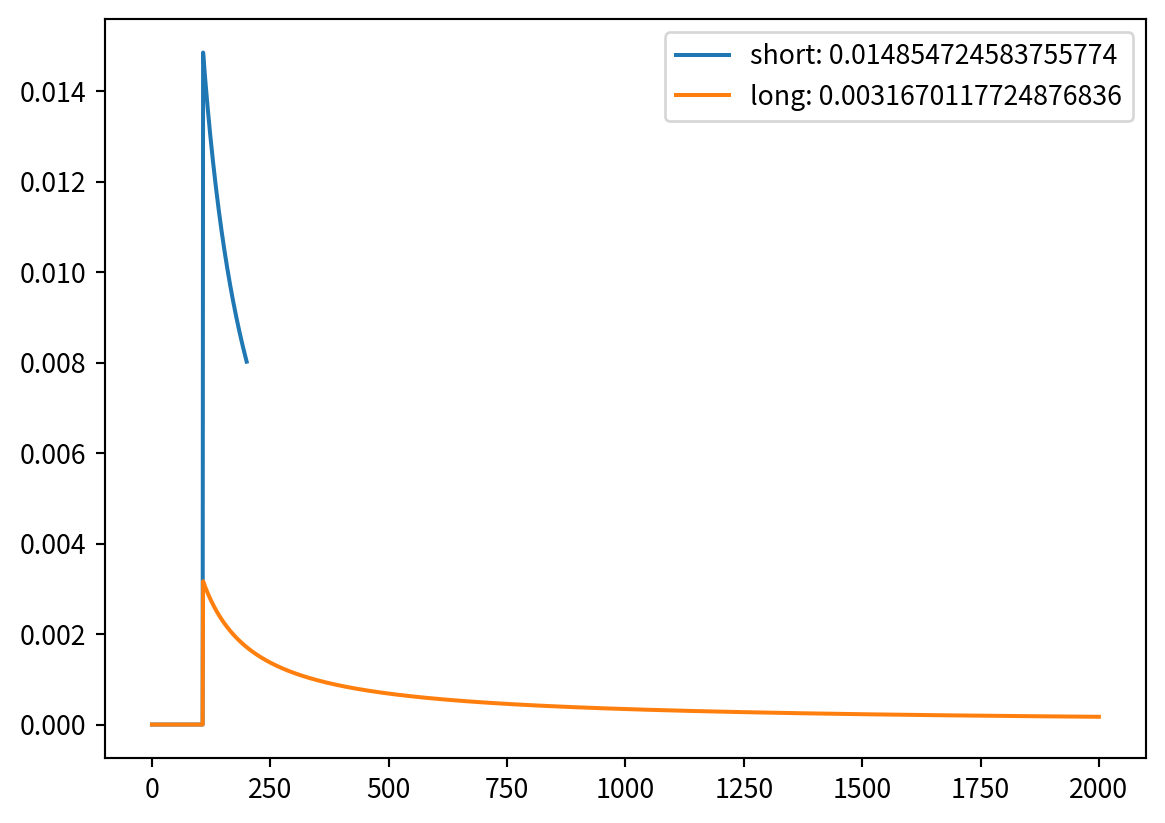
prior = Pmf.from_seq(['short', 'long'])
for hypos in prior.index:
    prior.loc[hypos] *= likelihood_ps[hypos]

prior.normalize()
prior| probs | |
|---|---|
| long | 0.175733 |
| short | 0.824267 |