확률보행

확률 통계
시계열 분석
공개

2025년 7월 9일

what is 확률보행

  • 확률보행: 무작위로 상승 또는 하락이 발생할 확률이 동일한 프로세스
    • \(y_t = C + y_{t-1} + ϵ_t\)
    • C가 0이 아닌 경우 표류가 있는 확률보행
import numpy as np
import matplotlib.pyplot as plt
import seaborn as sns

plt.rcParams['font.family'] = 'Noto Sans KR'

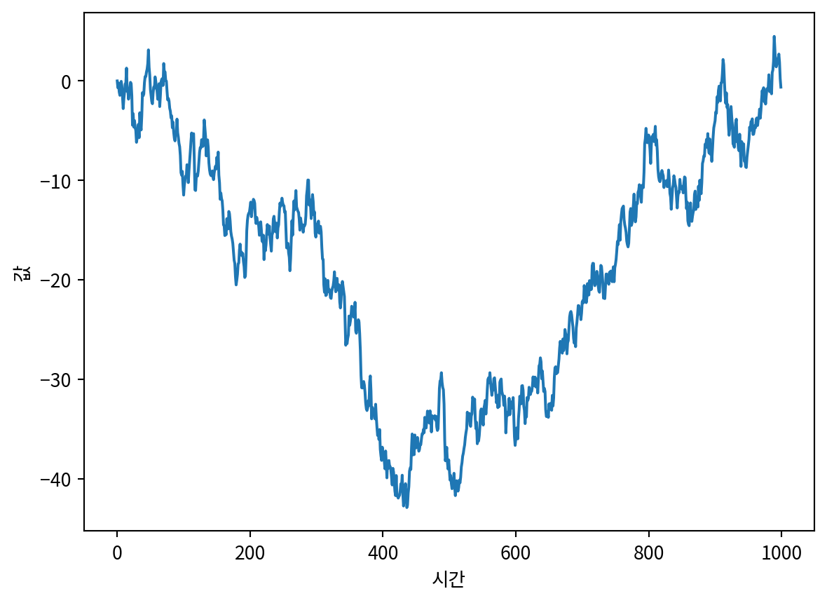
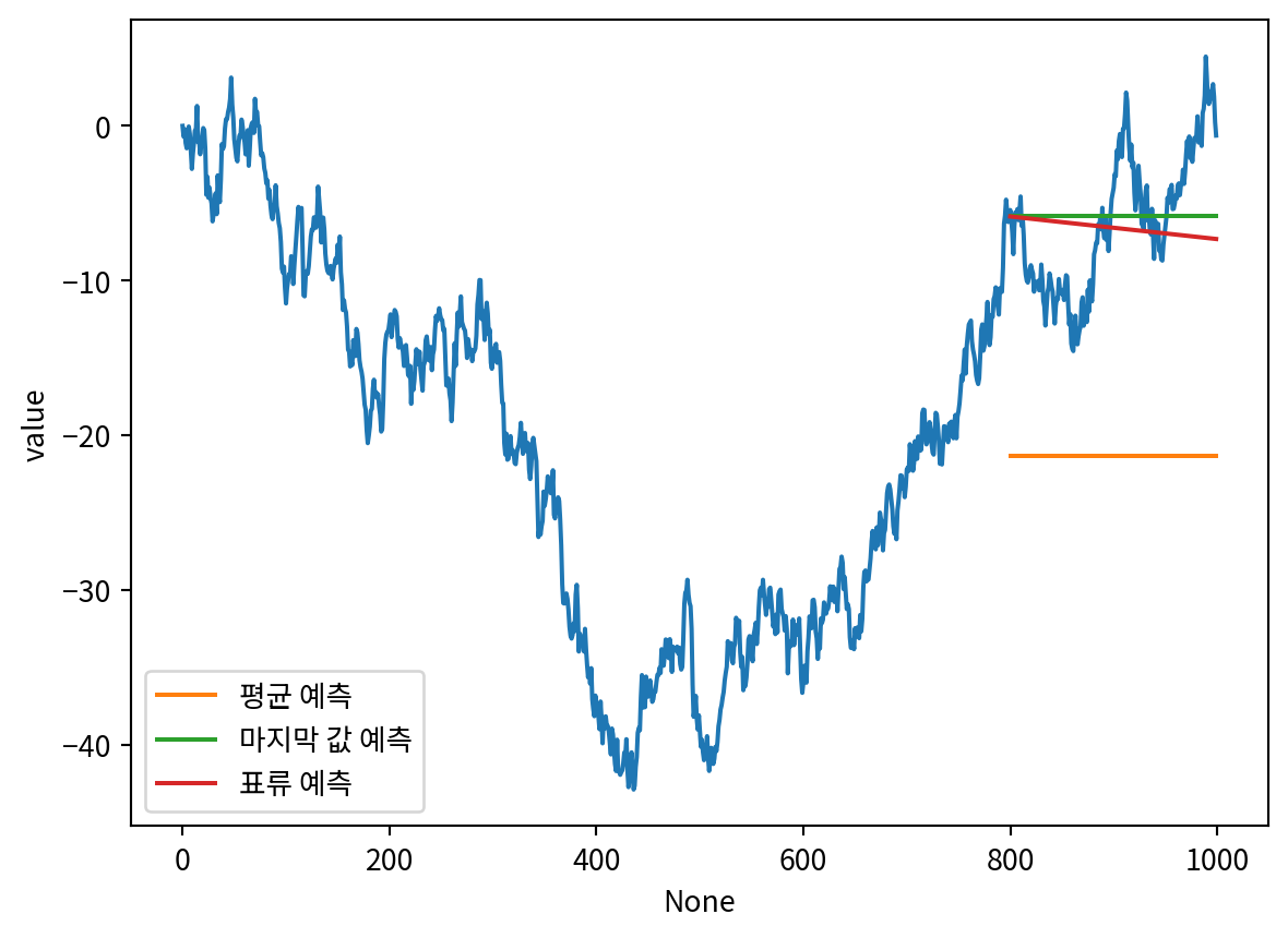
steps = np.random.standard_normal(1000)
steps[0] = 0
random_walk = np.cumsum(steps)
sns.lineplot(x=np.arange(len(random_walk)), y=random_walk)
plt.xlabel('시간')
plt.ylabel('값')
Text(0, 0.5, '값')

확률보행 식별

  • 확률보행은 정상적이고 자기상관관계가 없는 시계열로 나타난다.

정상성

  • 시간이 지나도 통계적 특성이 변하지 않는 시계열
    • 평균과 분산이 상수이고 자기상관관계가 있으며, 이러한 특성들이 시간에 따라 변하지 않는다.
  • 정상화:
    • 평균: 차분
    • 분산: 로그 변환, Box-Cox 변환 등
  • 정상성 검정:
    • ADF (Augmented Dickey-Fuller) 테스트
      • \(H_0\): 시계열에 단위근1이 존재하여 비정상적이다.
      • \(H_1\): 시계열에 단위근이 존재하지 않아 정상적이다.
import numpy as np
from statsmodels.tsa.stattools import adfuller

def simulate_process(alpha: float) -> np.array:
    process = np.empty(401)
    process[0] = 0
    for i in range(400):
        process[i+1] = alpha * process[i] + np.random.standard_normal()
    return process

stationary = simulate_process(alpha=0.5)
non_stationary = simulate_process(alpha=1)

sns.lineplot(x=np.arange(len(stationary)), y=stationary, label='정상성 프로세스')
sns.lineplot(x=np.arange(len(non_stationary)), y=non_stationary, label='비정상성 프로세스')

def mean_var_over_time(process: np.array) -> np.array:
    means = []
    vars = []
    for i in range(len(process)):
        means.append(np.mean(process[:i]))
        vars.append(np.var(process[:i]))
    return means, vars

means_stationary, vars_stationary = mean_var_over_time(stationary)
means_non_stationary, vars_non_stationary = mean_var_over_time(non_stationary)

sns.lineplot(x=np.arange(len(means_stationary)), y=means_stationary, label='정상성 평균')
sns.lineplot(x=np.arange(len(means_non_stationary)), y=means_non_stationary, label='비정상성 평균')

sns.lineplot(x=np.arange(len(vars_stationary)), y=vars_stationary, label='정상성 분산')
sns.lineplot(x=np.arange(len(vars_non_stationary)), y=vars_non_stationary, label='비정상성 분산')

result1 = adfuller(stationary)
result2 = adfuller(non_stationary)
print(f'ADF Statistic: 정상성: {result1[0]}, 비정상성: {result2[0]}')
print(f'p-value: 정상성: {result1[1]}, 비정상성: {result2[1]}')
ADF Statistic: 정상성: -10.182654946345801, 비정상성: -2.2791893442991604
p-value: 정상성: 6.632269182398948e-18, 비정상성: 0.17876768439598817

자기상관관계

  • 자기 상관관계: 시계열의 선행값과 후행값 아이의 선형관계
    • x: 지연 (\(y_t, y_{t-2}\)의 경우 지연 2)
    • y: 계수
  • 추세가 있는 경우: 짧은 지연에서 계수가 높고, 지연이 커질수록 계수가 낮아지는 경향
  • 계절성이 있는 경우: 주기적인 패턴이 나타남.
from statsmodels.graphics.tsaplots import plot_acf

plot_acf(non_stationary, lags=20)

  • 비정상적 시계열에서 추세가 보인다. 차분을 진행해보자.
diff = np.diff(non_stationary, n=1)

result = adfuller(diff)
result[0], result[1]
(-19.871934314399926, 0.0)
plot_acf(diff, lags=20)

예시

import pandas as pd

df = pd.read_csv('_data/googl.csv')
sns.lineplot(data=df, x='Date', y='Close')

plt.xlabel('날짜')
plt.ylabel('종가')

plt.xticks([4, 24, 46, 68, 89, 110, 132, 152, 174, 193, 212, 235],
           ['May', 'Jun', 'Jul', 'Aug', 'Sep', 'Oct', 'Nov', 'Dec', 'Jan', 'Feb', 'Mar', 'Apr'],
           rotation=45)
plt.show()

result = adfuller(df['Close'])

result[0], result[1]
(0.16025048664771407, 0.9699419435913058)
diff = np.diff(df['Close'], n=1)

result_diff = adfuller(diff)
result_diff[0], result_diff[1]
(-5.303439704295227, 5.386530961454778e-06)
plot_acf(diff, lags=20)

확류보행 예측

df = pd.DataFrame({'value': random_walk})
train = df.iloc[:800]
test = df.iloc[800:]

mean = np.mean(train['value'])
test['pred_mean'] = mean

last_value = train.iloc[-1]['value']
test['pred_last'] = last_value

표류 기법

drift = (train.iloc[-1]['value'] - train.iloc[0]['value']) / (len(train) - 1)
drift
-0.0073114182124709975
x_vals = np.arange(801, 1001)
pred_drift = drift * x_vals
test['pred_drift'] = pred_drift
sns.lineplot(data=df, x=df.index, y='value')
sns.lineplot(data=test, x=test.index, y='pred_mean', label='평균 예측')
sns.lineplot(data=test, x=test.index, y='pred_last', label='마지막 값 예측')
sns.lineplot(data=test, x=test.index, y='pred_drift', label='표류 예측')

from sklearn.metrics import mean_squared_error

mse_mean = mean_squared_error(test['value'], test['pred_mean'])
mse_last = mean_squared_error(test['value'], test['pred_last'])
mse_drift = mean_squared_error(test['value'], test['pred_drift'])

sns.barplot(x=['평균', '마지막 값', '표류'], y=[mse_mean, mse_last, mse_drift])

단순 예측법

df_shift = df.shift(periods=1)
mse_one_step = mean_squared_error(test['value'], df_shift['value'].iloc[800:])
mse_one_step
1.0373151143278658
맨 위로

각주

  1. \(y_t = C + αy_{t-1} + ϵ_t\) 형태의 시계열로, α가 1보다 작은 경우, 과거의 값이 현재 값에 미치는 영향이 작아져 시계열이 정상적이다.↩︎