복잡한 시계열 모델

확률 통계

시계열 분석

공개

2025년 7월 11일

from statsmodels.tsa.arima_process import ArmaProcess
import numpy as np
import pandas as pd
import matplotlib.pyplot as plt
import seaborn as sns

plt.rcParams['font.family'] = 'Noto Sans KR'

ar1 = np.array([1, -0.33])
ma1 = np.array([1, 0.9])

ARMA_1_1 = ArmaProcess(ar1, ma1).generate_sample(nsample=1000)

from statsmodels.tsa.stattools import adfuller

ADF_result = adfuller(ARMA_1_1)

ADF_result[0], ADF_result[1]

(-7.656346674014989, 1.7349289952389427e-11)

from statsmodels.graphics.tsaplots import plot_acf, plot_pacf

plot_acf(ARMA_1_1, lags=20)
plt.show()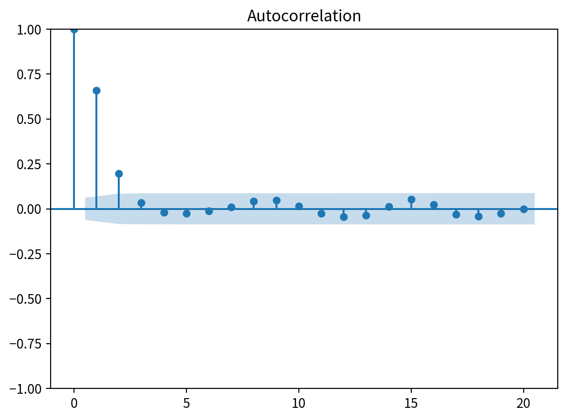

ARMA(1, 1) 모델인데 지연이 2.
ACF로는 차수를 추론할 수 없음.

plot_pacf(ARMA_1_1, lags=20)
plt.show()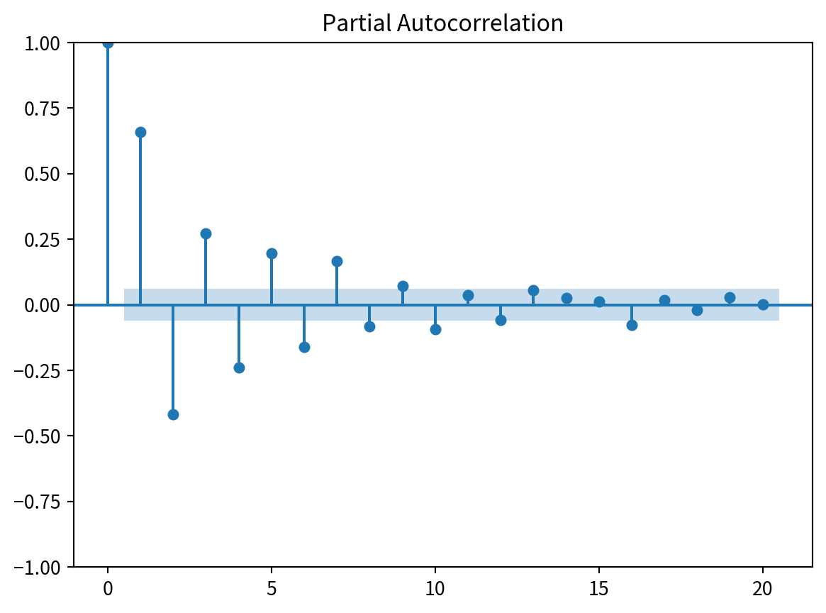

마찬가지로 차수를 추론할 수 없음.

일반적 모델링 절차

\(AIC = 2k - 2ln(\hat{L})\)
k = p + q
L = max(likelihood)

from itertools import product

ps = range(0, 4, 1)
qs = range(0, 4, 1)

order_list = list(product(ps, qs))

from typing import Union
from statsmodels.tsa.statespace.sarimax import SARIMAX

def optimize_ARMA(endog: Union[pd.Series, list], order_list: list) -> pd.DataFrame:
    results = []
    for order in order_list:
        try:
            model = SARIMAX(endog, order=(order[0], 0, order[1]), simple_differencing=False).fit(disp=False)
        except:
            continue
        aic = model.aic
        results.append([order, aic])
    result_df = pd.DataFrame(results)
    result_df.columns = ['(p, q)', 'AIC']
    result_df = result_df.sort_values(by="AIC").reset_index(drop=True)

    return result_df

result_df = optimize_ARMA(ARMA_1_1, order_list)
result_df

/home/cryscham123/.local/lib/python3.12/site-packages/statsmodels/base/model.py:607: ConvergenceWarning:

Maximum Likelihood optimization failed to converge. Check mle_retvals

	(p, q)	AIC
0	(1, 2)	2880.745326
1	(2, 2)	2881.184850
2	(2, 1)	2881.215973
3	(0, 3)	2881.552804
4	(0, 2)	2881.934005
5	(1, 1)	2882.021239
6	(1, 3)	2882.411069
7	(3, 1)	2882.880564
8	(2, 3)	2883.178911
9	(3, 3)	2884.999545
10	(3, 2)	2885.215581
11	(0, 1)	2998.204843
12	(3, 0)	3059.234951
13	(2, 0)	3135.429791
14	(1, 0)	3326.498642
15	(0, 0)	3894.252408

잔차 분석

model = SARIMAX(ARMA_1_1, order=(1, 0, 1), simple_differencing=False)
model_fit = model.fit(disp=False)

model_fit.plot_diagnostics(figsize=(12, 8))
plt.show()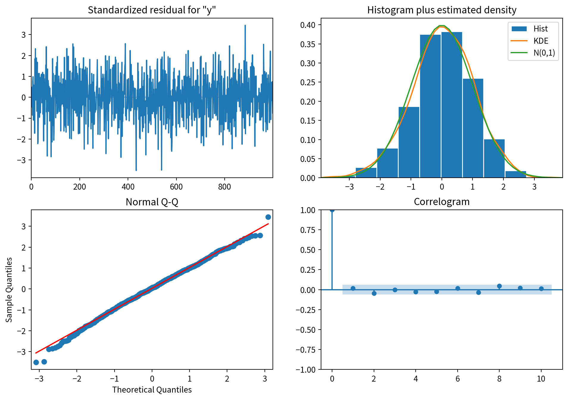

from statsmodels.stats.diagnostic import acorr_ljungbox

tr = acorr_ljungbox(model_fit.resid, np.arange(1, 11))
print(tr)

     lb_stat  lb_pvalue
1   0.289153   0.590764
2   2.289623   0.318284
3   2.291207   0.514207
4   2.963817   0.563899
5   3.571527   0.612593
6   3.938499   0.684999
7   5.248137   0.629711
8   7.642936   0.469103
9   8.139031   0.520198
10  8.329570   0.596679

예시 - 대역폭 사용량 예측

df = pd.read_csv('_data/bandwidth.csv')
sns.lineplot(data=df, x=df.index, y='hourly_bandwidth')

plt.xlabel('시간')
plt.ylabel('시간당 대역폭 사용량(MBps)')
plt.xticks(
    np.arange(0, 10000, 730), 
    ['Jan', 'Feb', 'Mar', 'Apr', 'May', 'Jun', 'Jul', 'Aug', 'Sep', 'Oct', 'Nov', 'Dec', '2020', 'Feb'])
plt.show()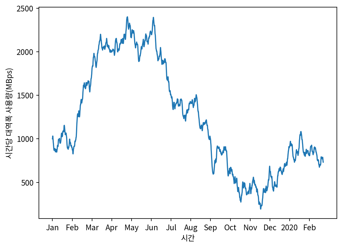

ADF_result = adfuller(df['hourly_bandwidth'])

ADF_result[0], ADF_result[1]

(-0.8714653199452845, 0.7972240255014515)

bandwidth_diff = np.diff(df['hourly_bandwidth'], n=1)

ADF_result = adfuller(bandwidth_diff)

ADF_result[0], ADF_result[1]

(-20.694853863789028, 0.0)

df_diff = pd.DataFrame({'bandwidth_diff': bandwidth_diff})
train = df_diff.iloc[:-168]
test = df_diff.iloc[-168:]

ps = range(0, 4, 1)
qs = range(0, 4, 1)
order_list = list(product(ps, qs))
result_df = optimize_ARMA(train['bandwidth_diff'], order_list)
result_df

	(p, q)	AIC
0	(3, 2)	27991.063879
1	(2, 3)	27991.287509
2	(2, 2)	27991.603598
3	(3, 3)	27993.416924
4	(1, 3)	28003.349550
5	(1, 2)	28051.351401
6	(3, 1)	28071.155496
7	(3, 0)	28095.618186
8	(2, 1)	28097.250766
9	(2, 0)	28098.407664
10	(1, 1)	28172.510044
11	(1, 0)	28941.056983
12	(0, 3)	31355.802141
13	(0, 2)	33531.179284
14	(0, 1)	39402.269523
15	(0, 0)	49035.184224

model = SARIMAX(train['bandwidth_diff'], order=(2, 0, 2), simple_differencing=False)
model_fit = model.fit(disp=False)
model_fit.plot_diagnostics(figsize=(12, 8))

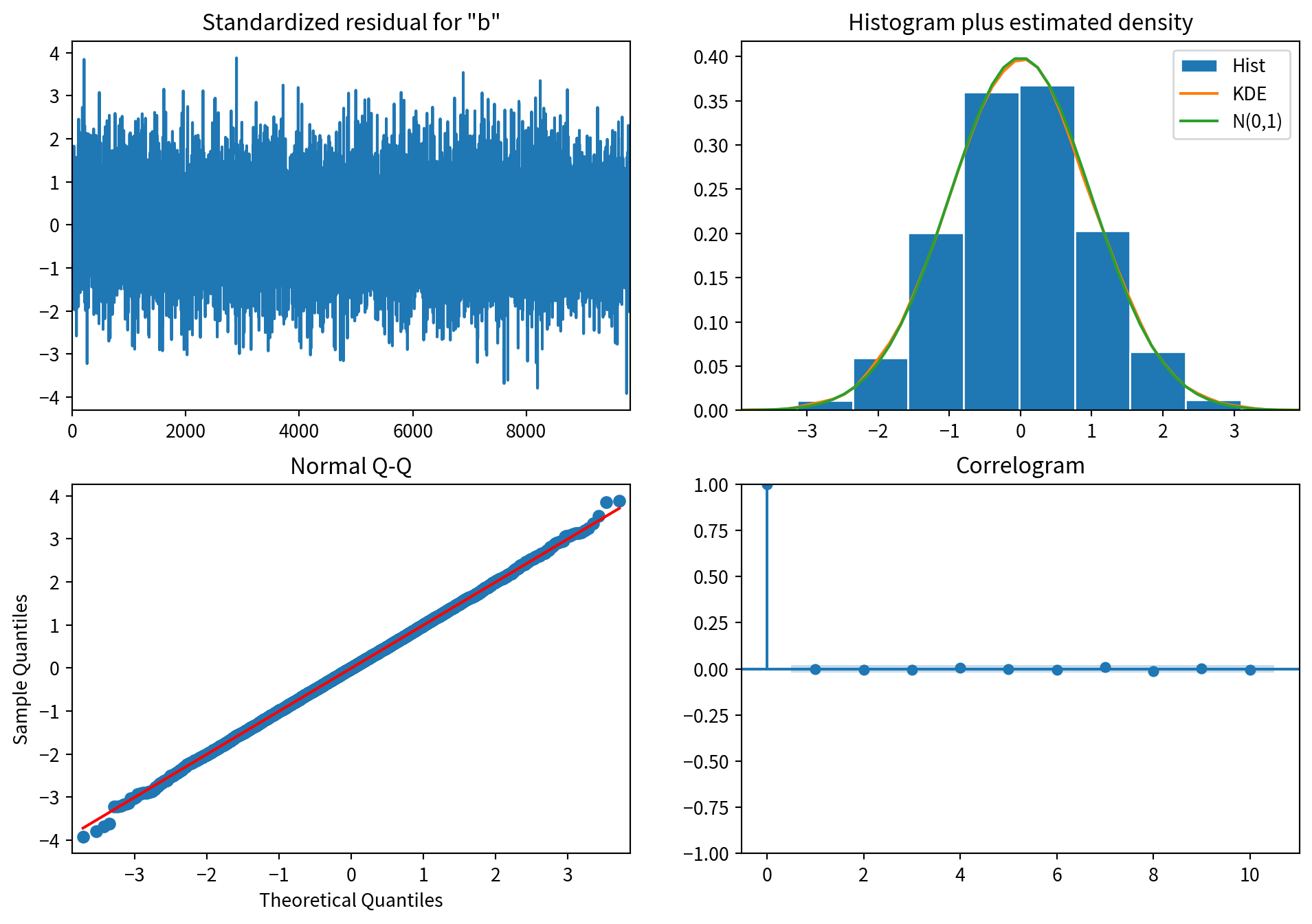
acorr_ljungbox(model_fit.resid, np.arange(1, 11))

	lb_stat	lb_pvalue
1	0.042190	0.837257
2	0.418364	0.811247
3	0.520271	0.914416
4	0.850554	0.931545
5	0.850841	0.973678
6	1.111754	0.981019
7	2.124864	0.952607
8	3.230558	0.919067
9	3.248662	0.953615
10	3.588289	0.964015

def rolling_forecast(df: pd.DataFrame, train_len: int, horizon: int, window: int, method: str) -> list:
    total_len = train_len + horizon
    if method == 'mean':
        pred_mean = []
        for i in range(train_len, total_len, window):
            mean = np.mean(df[:i].values)
            pred_mean.extend(mean for _ in range(window))
        return pred_mean
    if method == 'last':
        pred_last_value = []
        for i in range(train_len, total_len, window):
            last_value = df.iloc[i-1].values[0]
            pred_last_value.extend(last_value for _ in range(window))
        return pred_last_value
    if method == 'ARMA':
        pred_MA = []
        for i in range(train_len, total_len, window):
            model = SARIMAX(df[:i], order=(2,0,2))
            res = model.fit(disp=False)
            predictions = res.get_prediction(0, i + window - 1)
            oos_pred = predictions.predicted_mean.iloc[-window:]
            pred_MA.extend(oos_pred)
        return pred_MA

pred_df = test.copy()
TRAIN_LEN = len(train)
HORIZON = len(test)
WINDOW = 2

pred_mean = rolling_forecast(df_diff, TRAIN_LEN, HORIZON, WINDOW, 'mean')
pred_last = rolling_forecast(df_diff, TRAIN_LEN, HORIZON, WINDOW, 'last')
pred_ARMA = rolling_forecast(df_diff, TRAIN_LEN, HORIZON, WINDOW, 'ARMA')

pred_df['pred_mean'] = pred_mean
pred_df['pred_last'] = pred_last
pred_df['pred_ARMA'] = pred_ARMA

sns.lineplot(data=pred_df, x=pred_df.index, y='bandwidth_diff', label='실제값')
sns.lineplot(data=pred_df, x=pred_df.index, y='pred_mean', label='평균 예측')
sns.lineplot(data=pred_df, x=pred_df.index, y='pred_last', label='마지막 값 예측')
sns.lineplot(data=pred_df, x=pred_df.index, y='pred_ARMA', label='ARMA(2, 2) 예측')
plt.xlabel('시간')
plt.ylabel('시간당 대역폭 사용량(MBps)')
plt.xticks(
    [9802, 9850, 9898, 9946, 9994],
    ['2020-02-13', '2020-02-15', '2020-02-17', '2020-02-19', '2020-02-21'])
plt.xlim(9800, 9999)
plt.show()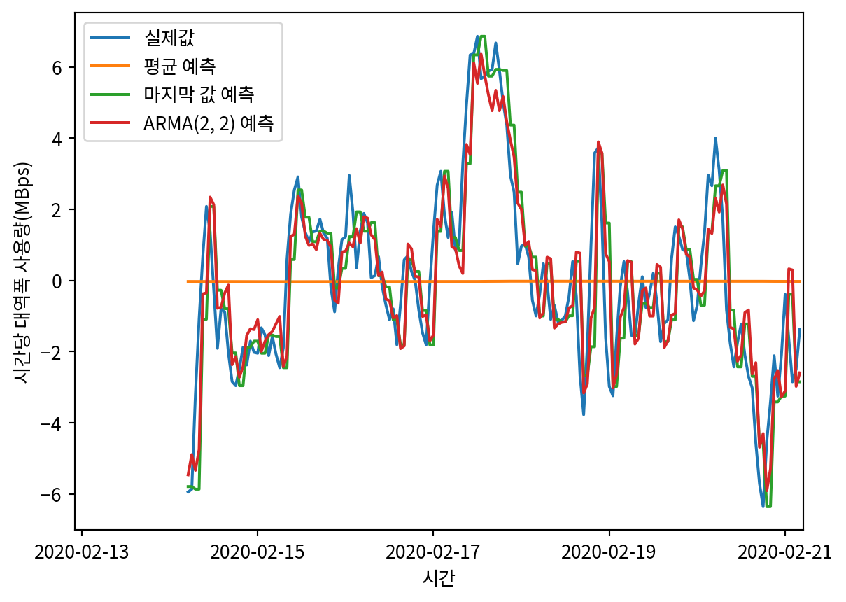

from sklearn.metrics import mean_squared_error, mean_absolute_error

mse_mean = mean_squared_error(pred_df['bandwidth_diff'], pred_df['pred_mean'])
mse_last = mean_squared_error(pred_df['bandwidth_diff'], pred_df['pred_last'])
mse_ARMA = mean_squared_error(pred_df['bandwidth_diff'], pred_df['pred_ARMA'])
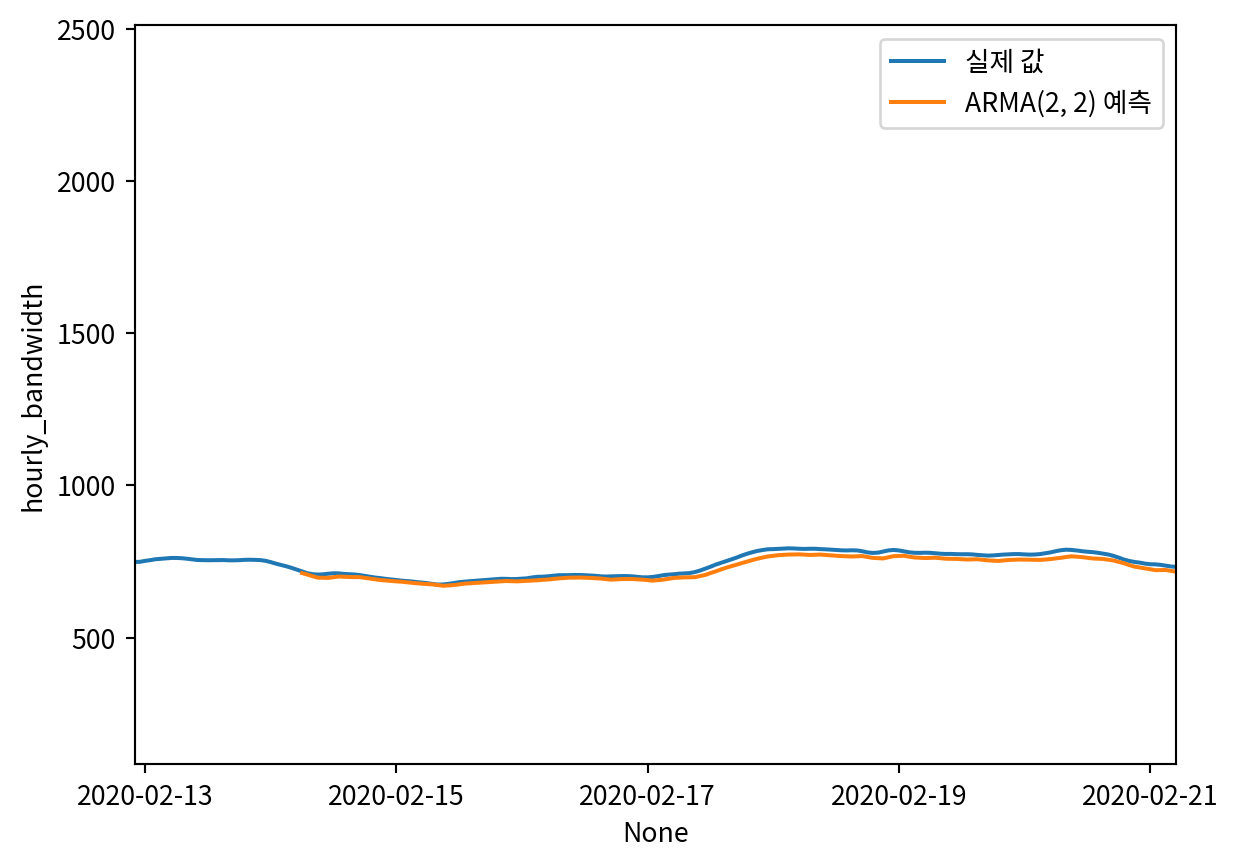
mse_mean, mse_last, mse_ARMA

(6.306526957989325, 2.2297582947733656, 1.7690462113874967)

역변환

df['pred_bandwidth'] = pd.Series()
df['pred_bandwidth'].iloc[9832:] = df['hourly_bandwidth'].iloc[9832] + pred_df['pred_ARMA'].cumsum()

sns.lineplot(data=df, x=df.index, y='hourly_bandwidth', label='실제 값')
sns.lineplot(data=df, x=df.index, y='pred_bandwidth', label='ARMA(2, 2) 예측')
plt.xticks(
    [9802, 9850, 9898, 9946, 9994],
    ['2020-02-13', '2020-02-15', '2020-02-17', '2020-02-19', '2020-02-21'])
plt.xlim(9800, 9999)
plt.show()

맨 위로