시계열 분석
데이터 분석
구성 요소
추세(level)계절, 순한: 추세에서 벗어나는 변화의 정도잔차(white noise)
EDA
df_isna = df.asfreq('H') # 시간 기준 결측치 탐색. index가 datetime이어야 함
df_isna[df_isna.isnull().any(axis=1)]
from statsmodels.tsa.seasonal import STL
decomposition = STL(df_final['value'], period=24).fit() # period는 계절성 주기
fig, (ax1, ax2, ax3, ax4) = plt.subplots(nrows=4, ncols=1, sharex=True, figsize=(10, 8))
ax1.plot(decomposition.observed)
ax1.set_ylabel('Obseved')
ax2.plot(decomposition.trend)
ax2.set_ylabel('Trend')
ax3.plot(decomposition.seasonal)
ax3.set_ylabel('Seasonal')
ax4.plot(decomposition.resid)
ax4.set_ylabel('Residuals')
plt.show()예측 방법
Rolling Forecast (동적 예측): - 각 시점에서 예측을 수행한 후, 실제 값이 관측되면 이를 학습 데이터에 추가하여 다음 시점을 예측 - 실제 운영 환경을 시뮬레이션하는 방법으로, 새로운 정보가 지속적으로 업데이트됨 - 장점: 최신 정보를 반영하여 더 정확한 예측 가능 - 단점: 계산 비용이 높고, 모델 성능 평가 시 과적합 위험
Static Forecast (정적 예측): - 초기 학습 데이터로만 모델을 한 번 학습하고, 이후 테스트 기간 전체에 대해 연속적으로 예측 - 고정된 모델로 여러 시점을 예측하므로 모델의 일반화 성능을 더 엄격하게 평가 - 장점: 계산 비용이 낮고, 공정한 모델 평가 가능 - 단점: 시간이 지날수록 예측 정확도가 떨어질 수 있음
단순 기법
- 단순예측법: 최근의 자료가 미래에 대한 최선의 추정치 \(\hat{p_{t+1}} = p_t\)
- 추세분석: 전기와 현기 사이의 추세를 다음 기의 판매예측에 반영하는 방법. \(\hat{p_{t+1}} = p_t + p_t - p_{t-1}\)
- 단순 이동평균법: time window를 계속 이동하면서 평균 구하는거
- time window ↑: 먼 과거까지 보겠다
- 가중 이동평균법: 가중치를 다르게 부여한 단순이동평균법
단순 기법 rolling forecast
def rolling_forecast_simple(train_data, test_data, method='naive'):
    predictions = []
    train_extended = train_data.copy()

    for i in range(len(test_data)):
        if method == 'naive':
            # 단순예측법: 마지막 값
            pred = train_extended.iloc[-1]['data']

        elif method == 'trend':
            # 추세분석법
            pred = train_extended.iloc[-1]['data'] + (train_extended.iloc[-1]['data'] - train_extended.iloc[-2]['data'])

        elif method == 'ma_4':
            # 4기간 이동평균
            pred = np.mean(train_extended.iloc[-4:]['data'])

        elif method == 'ma_12':
            # 12기간 이동평균
            window = min(12, len(train_extended))
            pred = np.mean(train_extended.iloc[-window:]['data'])

        elif method == 'seasonal_naive':
            # 계절 단순예측법 (4분기 전과 동일)
            if len(train_extended) >= 4:
                pred = train_extended.iloc[-4]['data']
            else:
                pred = train_extended.iloc[-1]['data']

        predictions.append(pred)

        # 실제 값을 train에 추가 (rolling)
        actual_value = test_data.iloc[i]
        train_extended = pd.concat([train_extended, actual_value.to_frame().T], ignore_index=True)

    return predictions

# 각 방법별 rolling forecast 수행
methods = ['naive', 'trend', 'ma_4', 'ma_12', 'seasonal_naive']
rolling_results = {}

for method in methods:
    predictions = rolling_forecast_simple(train, test, method)
    rolling_results[method] = predictions

# 결과를 DataFrame으로 정리
results_df = pd.DataFrame(rolling_results)
results_df['actual'] = test['data'].values
results_df.index = test.index
print(results_df)
지수 평활법

- α -> 1: 최근 자료에 비중을 둠. α -> 0: 기존 예측을 따름
지수 평활법 rolling forecast
from statsmodels.tsa.holtwinters import SimpleExpSmoothing

def rolling_forecast_exponential_smoothing(train_data, test_data, a=0.5):
    predictions = []
    train_extended = train_data.copy()

    for i in range(len(test_data)):
        try:
            # 모델 적합
            model = SimpleExpSmoothing(train_extended['value'])
            model_fit = model.fit(smoothing_level=a, optimized=False)

            # 예측
            pred = model_fit.predict(len(train_extended))
            predictions.append(pred.iloc[0])

        except Exception as e:
            print(f"Error at step {i}: {e}")
            # 오류 발생시 naive 예측 사용
            predictions.append(train_extended.iloc[-1]['value'])

        # 실제 값을 train에 추가 (rolling)
        actual_value = test_data.iloc[i]
        train_extended = pd.concat([train_extended, actual_value.to_frame().T], ignore_index=True)

    return predictions

# 지수 평활법 rolling forecast 실행 예시
exp_smooth_predictions = rolling_forecast_exponential_smoothing(train, test, a=0.3)
SARIMAX 계열
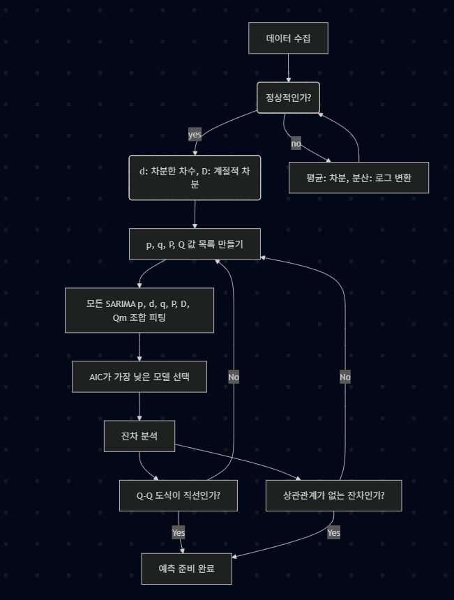
정상성 확인
- 정상시계열은 분산과 평균, 자기 상관이 시간에 따라 변하지 않는 시계열
- 분산이 일정하지 않은 경우: 로그 변환
- 그래프로 확인
- 평균이 일정하지 않은 경우: 차분
stationarity test
from statsmodels.tsa.stattools import adfuller

ad_fuller_result = adfuller(df['value'])

print('ADF Statistic:', ad_fuller_result[0])
print('p-value:', ad_fuller_result[1])- p-value < 0.05: 귀무가설 기각, 정상시계열
- 주로 평균이 일정하지 않은 것을 찾아낼 수 있다.
difference
df = df.diff()- 만약 차분 후에도 정상성이 만족되지 않는다면, 계절 차분을 고려
seasonal difference
df = df.diff(12) # 12개월 주기from statsmodels.graphics.tsaplots import plot_acf, plot_pacf
plot_acf(df['value'].dropna(), lags=30)
plot_pacf(df['value'].dropna(), lags=30)
plt.show()- 자기 상관이 존재하는 경우
- ACF, PACF 그래프로 확인
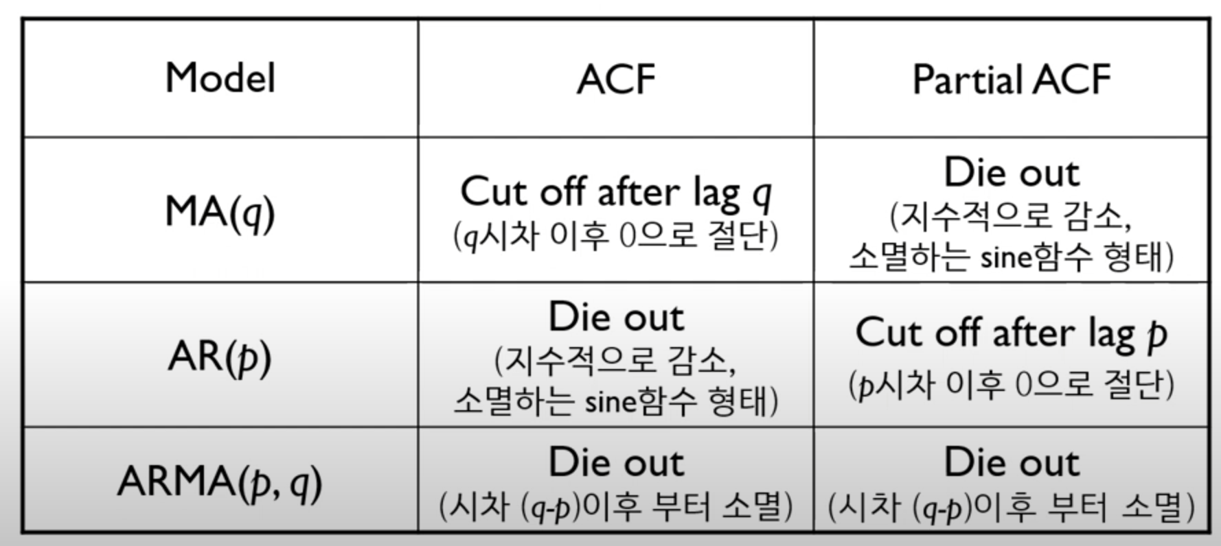
- 하지만 매우 주관적일 수 있으므로, 직접 여러 모델을 돌려본 후 AIC 기준으로 선택.
- 그리고 다시 검정 진행
SARIMAX 모델 적합
SARIMAX
from statsmodels.tsa.statespace.sarimax import SARIMAX
from itertools import product

p = range(0, 4, 1)
d = 1 # 차분 횟수
q = range(0, 4, 1)
P = range(0, 4, 1)
D = 0 # 계절 차분 횟수
Q = range(0, 4, 1)
s = 4 # 계절 주기
parameters = product(p, q, P, Q)
order_list = list(parameters)

results = []
for order in order_list:
    try:
        model = SARIMAX(train['value'],
                        exog,
                        order=(order[0], d, order[1]),
                        seasonal_order=(order[2], D, order[3], s),
                        simple_differencing=False).fit(disp=False)
    except:
        continue
    aic = model.aic
    results.append([order, aic])
results_df = pd.DataFrame(results, columns=['(p, q, P, Q)', 'AIC'])
results_df = results_df.sort_values(by='AIC', ascending=True).reset_index(drop=True)
display(results_df)
best_model = SARIMAX(train['value'],
exog,
order=(2, 1, 2), # [2, 3], 0, 1 이런 식으로도 가능(y_t-2, y_t-3 사용하는 방법)
simple_differencing=False).fit(disp=False)best_model.summary()- 결과 확인
best_model.plot_diagnostics(figsize=(10, 8))
plt.show()- 등분산성, 정규성 만족하는지 육안으로 확인
ljung-box
from statsmodels.stats.diagnostic import acorr_ljungbox

ljung_box_result = acorr_ljungbox(best_model.resid, lags=[10], return_df=True)
print(ljung_box_result)- p-value가 0.05보다 크면 잔차가 백색잡음
SARIMAX rolling forecast
def rolling_forecast_sarimax(train_data, test_data, order, seasonal_order, exog_train=None, exog_test=None):
    predictions = []
    train_extended = train_data.copy()
    exog_extended = exog_train.copy() if exog_train is not None else None

    for i in range(len(test_data)):
        try:
            # 모델 적합
            if exog_extended is not None:
                model = SARIMAX(train_extended['value'],
                               exog=exog_extended,
                               order=order,
                               seasonal_order=seasonal_order,
                               simple_differencing=False)
            else:
                model = SARIMAX(train_extended['value'],
                               order=order,
                               seasonal_order=seasonal_order,
                               simple_differencing=False)
            model_fit = model.fit(disp=False)
            # 예측
            if exog_test is not None:
                pred = model_fit.forecast(steps=1, exog=exog_test.iloc[i:i+1])
            else:
                pred = model_fit.forecast(steps=1)
            predictions.append(pred.iloc[0])
        except Exception as e:
            print(f"Error at step {i}: {e}")
            # 오류 발생시 naive 예측 사용
            predictions.append(train_extended.iloc[-1]['value'])

        # 실제 값을 train에 추가 (rolling)
        actual_value = test_data.iloc[i]
        train_extended = pd.concat([train_extended, actual_value.to_frame().T], ignore_index=True)

        if exog_extended is not None and exog_test is not None:
            exog_extended = pd.concat([exog_extended, exog_test.iloc[i:i+1]], ignore_index=True)

    return predictions

# SARIMAX rolling forecast 실행 예시
sarimax_predictions = rolling_forecast_sarimax(
    train, test,
    order=(2, 1, 2),
    seasonal_order=(0, 0, 0, 4)  # 계절성이 없는 경우
)